Synchronization
Synchronization in Distributed Systems
The Synchronization Problem
Core Challenges
- Lack of Shared Memory: Traditional synchronization methods (like semaphores) fail because they rely on shared memory, which doesn't exist in distributed systems.
- Event Ordering: Without a global clock or shared memory, it is difficult to determine which event occurred first (relative ordering).
- Goal: Processes must cooperate and synchronize using only message passing.
Physical Clocks & Time Measurement
How Computer Clocks Work
- Hardware Timer: Computers do not have "clocks"; they have "timers." A quartz crystal oscillates at a specific frequency, decrementing a hardware counter. When the counter hits zero, it triggers an interrupt (clock tick) and reloads from a holding register.
- Software Clock: The OS interrupt handler counts these ticks to maintain the current time.
Clock Skew
- Because crystals are not perfect, they oscillate at slightly different frequencies.
- Result: Over time, the software clocks of different machines will drift apart, even if they started at the exact same time. This divergence is called Clock Skew.
Global Time Standards
- Atomic Clocks: Highly accurate time measurement available in labs (e.g., Paris).
- TAI (Temps Atomique International): The average of atomic clocks worldwide.
- UTC (Universal Coordinated Time): The standard civil time used globally.
Clock Synchronization Logic
The "Make" Compilation Problem Discrepancies in time can break logic.
- Scenario: You edit
input.con machine A (Time: 2144) and compile it on machine B (Time: 2145). - The Error: If Machine A is slow and thinks it is 2142, it saves the source file with timestamp 2142. Machine B sees
input.o(2144) is "newer" thaninput.c(2142) and refuses to recompile, even though the source just changed.
Mathematical Model of Drift
- Definitions:
- \(t\): The actual "Real" time (UTC).
- \(C(t)\): The time shown by the computer's internal clock at real time \(t\).
- \(dC/dt\): The rate at which the computer clock advances relative to real time.
- Perfect Clock: \(dC/dt = 1\), like \(C_p(t)=t\) for all machines \(p\)
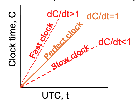
- Drift Rate (\(\rho\)): The maximum rate a clock can speed up or slow down (specified by the manufacturer, typically \(10^{-5}\) for modern chips).
- Formula: The clock drift is bounded by \(1-\rho \le dC/dt \le 1+\rho\).
- Resynchronization Interval: To keep two clocks within a maximum difference of \(\delta\), they must be resynchronized every \(\delta / 2\rho\) seconds (because they might drift in opposite directions).
Synchronization Algorithms
Cristian's Algorithm
- Setup: One machine acts as a Time Server (connected to a WWV receiver); all other machines act as clients that stay synchronized with it.
- The Process:
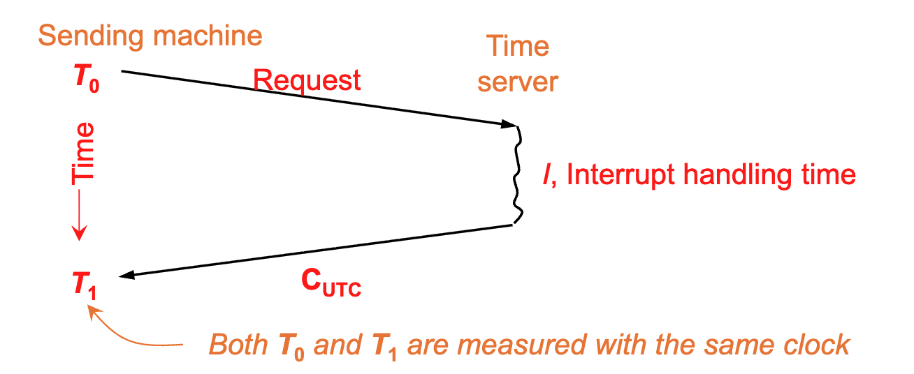
- Sending (\(T_0\)): The Client machine sends a request to the server. The timestamp \(T_0\) is recorded by the Client's clock.
- Interrupt (\(I\)): The Server receives the request and processes it (Interrupt handling time \(I\)).
- Reply (\(C_{UTC}\)): The Server sends back its current time (\(C_{UTC}\)).
- Receiving (\(T_1\)): The Client receives the reply. The timestamp \(T_1\) is recorded by the Client's clock.
- The Calculation:
- Goal: The client wants to set its clock to the Server's time, but the message took time to travel.
- Round Trip Time (RTT): \(RTT = T_1 - T_0\).
- New Time: The Client sets its time to: \(Server\_time + RTT/2\).
- Key Assumption: The algorithm assumes the network delay is symmetric, meaning the request and the reply took the exact same amount of time to travel (\(T_{req} \approx T_{res}\)).
- Gradual Adjustment: Changes are introduced gradually (by adding slightly more/less seconds per interrupt) rather than jumping time instantly.
- The propagation time is included in the change, which means the algorithm is compensating for the speed of light and network lag. It’s not just copying a number; it’s calculating the number + the delivery time so the clock is accurate the moment it is updated.
Network Time Protocol (NTP)
- Type: Symmetric / Peer-to-Peer.
- Scenario: Used over the internet to achieve high accuracy between machines B and A.
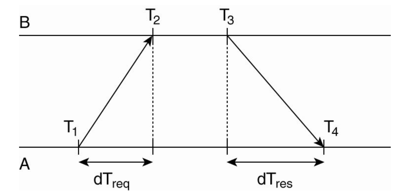
- Mechanism: Measures four timestamps across a request/reply pair:
- \(T_1\): A sends request.
- \(T_2\): B receives request.
- \(T_3\): B sends reply.
- \(T_4\): A receives reply.
- Offset Calculation: It calculates the time difference (Offset) between A and B while cancelling out the network delay:
- \(Offset = ((T_2 - T_1) + (T_3 - T_4)) / 2\).
- Action: The system gradually adjusts the clock to minimize this offset rather than jumping the time instantly (the clock will not go backward).
Global Time Standards (UTC)
Universal Coordinated Time (UTC)
- Definition: A global time standard corrected with "leap seconds" to account for the slowing of the earth's rotation (mean solar day getting longer).
- Sources for Precise Time:
- WWV (NIST): Shortwave radio station from Colorado. Accuracy: \(\pm 1\) msec.
- GEOS: Earth satellites. Accuracy: \(0.5\) msec.
- Telephone (NIST): Available via modem, but less accurate and cheaper.
Network Time Protocol (NTP)
Architecture
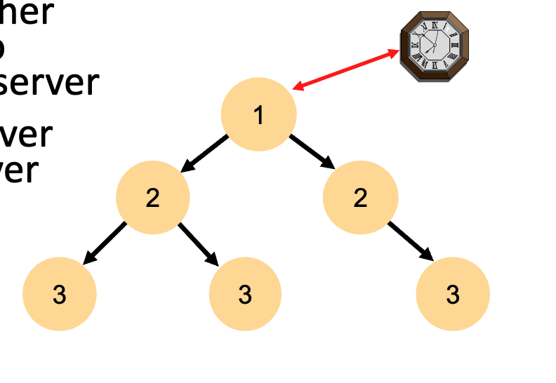
- Layered System: Uses a hierarchy of "Strata" based on UDP message passing.
- Stratum 1: Servers directly connected to a precision time source (like an atomic clock).
- Stratum 2: Servers that sync with Stratum 1, and so on. Accuracy decreases as the strata number increases due to network latency.
- As the stratum number increases, the accuracy slightly decreases because every "hop" over the network adds a little bit of latency (delay).
- Failure Robustness: If a Stratum 1 server fails, the hierarchy reconfigures automatically; a backup can become the new primary.
- "If a strata 1 server fails," it doesn't necessarily mean the whole computer exploded or turned off. In the world of NTP, "Failure" usually means loss of the time signal.
- If a Stratum 1 server loses its connection to its atomic clock, it doesn't just stop. It can "re-home" itself to another Stratum 1 server nearby.
- When it does this, it automatically drops down to become a Stratum 2 server. This ensures that time keeps flowing even during hardware failures.
Operational Modes
- Multicast: One computer periodically broadcasts time to a LAN.
- Procedure Call: Similar to Cristian's Algorithm (Client requests time \(\rightarrow\) Server replies).
The Berkeley Algorithm
Concept
- Type: Active Time Server (Centralized).
- Usage: Suitable when no machine has a WWV receiver/external source.
-
Mechanism:
- Polling: A central "Time Daemon" periodically asks every machine for its time.
- Averaging: The daemon computes the average time from all answers.
- Adjustment: It tells machines to advance or slow down their clocks to match the average.
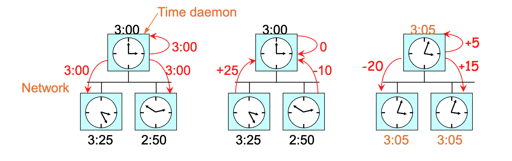
-
Constraint: If a clock is fast, it is instructed to slow down until the others catch up; time is never set backwards to avoid breaking software logic.
Decentralized Averaging Algorithm
Concept
- Type: Decentralized / Peer-to-Peer.
- Mechanism:
- Time is divided into fixed resynchronization intervals (\(R\)).
- At the start of an interval, every machine broadcasts its current time.
- At the beginning of each interval, each machine broadcasts the current time according to its own clock (broadcasts are not likely to happen simultaneously because the clocks on different machine do not run at exactly the same speed)
- After collecting broadcasts for a set time (\(S\)), each machine runs a local algorithm to compute the new time (typically averaging all values).
- If some broadcasts don't arrive within the time window S, the machine stops waiting and performs the calculation with whatever data it actually managed to collect.
- Variations: To improve accuracy, algorithms may discard the \(m\) highest and \(m\) lowest values (outliers) before averaging. Additionally, before computing new time, an estimate of the propagation time from the source can be added to each message to compensate for network latency.
Logical Clocks (Lamport Timestamps)
Physical vs. Logical
- Physical Clocks: Must not deviate from real-world time.
- Logical Clocks: Internal consistency matters more than real time. Processes only need to agree on the order in which events occur, not the time of day.
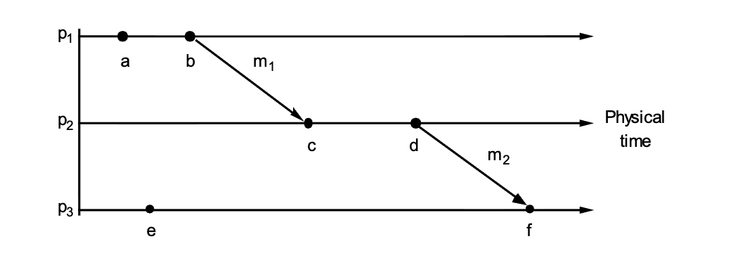
The "Happens-Before" Relation (\(\rightarrow\))
Defines ordering without a physical clock:
- Same Process: If \(a\) and \(b\) are in the same process and \(a\) occurs before \(b\), then \(a \rightarrow b\).
- Message Passing: If \(a\) is sending a message and \(b\) is receiving it, then \(a \rightarrow b\).
- Transitivity: If \(a \rightarrow b\) and \(b \rightarrow c\), then \(a \rightarrow c\).
- Concurrency: If neither \(a \rightarrow b\) nor \(b \rightarrow a\) is true, the events are Concurrent (\(a || b\)). Like they do not exchange messages
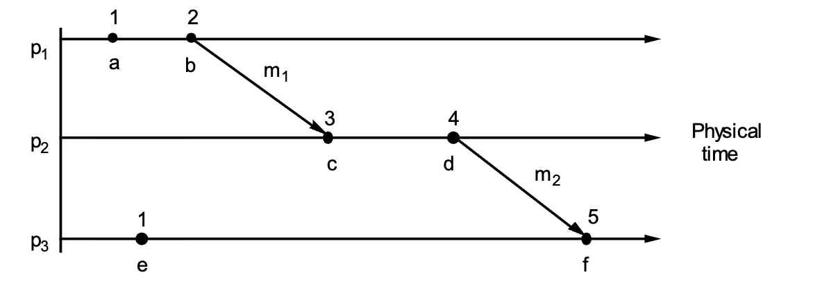
Lamport's Algorithm Rules
Every process \(P_i\) maintains a logical counter \(L_i\).
- Local Event: Before any event occurs, increment the counter: \(L_i := L_i + 1\).
- Sending: When sending message \(m\), attach the timestamp \(t = L_i\).
- Receiving: When receiving \((m, t)\), update the local clock to be greater than both the local time and the message time: \(L_j := \max(L_j, t) + 1\).
Total Ordering Solution
- Problem: Two events on different machines might end up with the same Lamport timestamp (e.g., both are 40).
- Solution: To differentiate them, append the Process ID as a decimal.
- Example: If Process 1 and Process 2 both have an event at time 40, they become 40.1 and 40.2. Since \(40.1 < 40.2\), the tie is broken arbitrarily but consistently.
1. The "Tick Every Event" Rule
Between every two events, the clock must tick at least once
To maintain a continuous timeline, a process must increment its counter (\(L\)) for every distinct action. This includes internal events (local computations, writing to a disk, or updating a variable), send events (preparing a message to leave the node), and receive events (accepting a message from the network). If Process 1 performs a local calculation and then immediately sends a message, those are two distinct states. If we didn't tick for the calculation, both the calculation and the message-send would have the same timestamp. This would break the "happens-before" relationship (\(a \to b\)), as we wouldn't be able to prove which one happened first.
2. The "No Two Events are Equal" Rule (Tie-Breaking)
No two events occur at exactly the same time. If two events happen in processes 1 and 2, both with time 40, the former becomes 40.1 and the latter becomes 40.2
Even with constant ticking, two different processes (\(P_1\) and \(P_2\)) might independently reach the same logical time (e.g., both reach \(T=40\)). To create a Total Order, we append the Process ID to the timestamp as a decimal. The formula for a global timestamp is \(L_i.i\). For example, Event A in \(P_1\) occurs at Logical Time 40 (Global Timestamp: 40.1) and Event B in \(P_2\) occurs at Logical Time 40 (Global Timestamp: 40.2). Because \(40.1 < 40.2\), the entire system agrees that Event A happened "before" Event B. Even though they happened at the same logical "moment," the Process ID acts as the ultimate tie-breaker.
3. Clock Synchronization (The Receive Rule)
When a message travels from \(P_1\) to \(P_2\), it carries the sender's timestamp (\(T_{send}\)). When \(P_2\) receives it, it must ensure its clock is "ahead" of the event that caused the message. The math used is \(L_{receiver} = \max(L_{receiver}, T_{send}) + 1\). For example, if \(P_1\) at Time \(10\) sends a message, it ticks to 11 and sends \(T=11\). If \(P_2\) is at Time \(5\) when the message arrives, simply ticking to \(6\) would make it look like the message was received before it was sent (\(6 < 11\)). Instead, \(P_2\) looks at the message (\(11\)), takes the Max (\(11\)), and ticks to \(12\). Now, the Send (\(11\)) correctly "happens-before" the Receive (\(12\)).
Total Ordering & Vector Clocks
Lamport Timestamps & Total Ordering
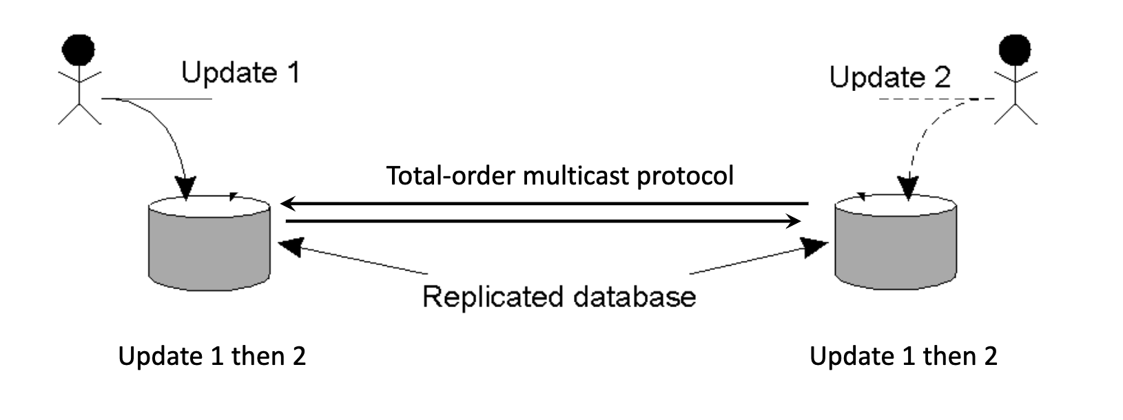
The Replicated Database Problem
-
Scenario: Two users update a replicated database simultaneously.
- User A sends "Update 1" to Replica 1.
- User B sends "Update 2" to Replica 2.
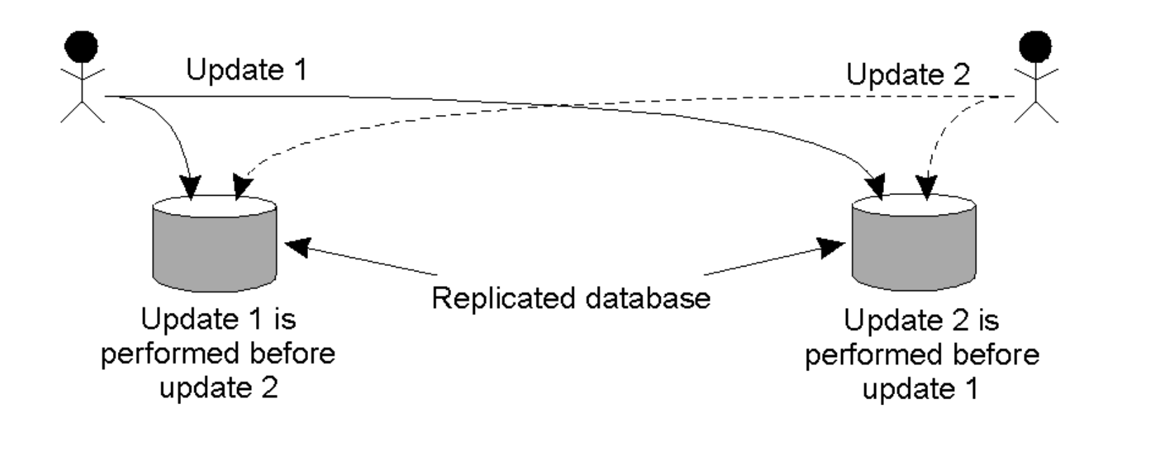
-
Conflict: If Replica 1 processes
1 -> 2and Replica 2 processes2 -> 1, the databases become inconsistent. - Requirement: Updates must be ordered the same way across all replicas (Total Ordering).
Total-Ordered Multicast Algorithm
Uses Lamport Clocks to ensure identical processing order.
- Sending: The sender adds its local logical timestamp to the message and broadcasts it to all nodes.
- Receiving: Nodes add the message to a local queue ordered by timestamp, update the local logical time and broadcast an Acknowledgment (Ack) to everyone.
- Delivery Rule: A message is only delivered to the application when:
- It is at the head of the queue.
- The node has received Acks for that message from all other nodes.
-
Result: Since all queues are ordered by the same timestamps, every node processes transactions in the exact same sequence.
The node has to receive the Ack which has the timestamp of the sender from all other nodes first, then verify all these timestamps are greater than or equal to the its head of the queue, and then the message can be delivered to the application.
Vector Clocks
Why Lamport Clocks Aren't Enough
Lamport clocks ensure total ordering but cannot distinguish whether events are causally related or concurrent (they lose the history). Vector Clocks solve this by capturing the entire causal history.
Structure & Properties
Each process \(P_i\) maintains a vector \(VC_i\) (an array of integers):
- \(VC_i[i]\): The number of events that have occurred locally at \(P_i\) (its own logical clock).
- \(VC_i[j]\): The number of events \(P_i\) knows have occurred at process \(P_j\).
- Knowledge: If \(VC_i[j] = k\), then Process \(i\) knows that Process \(j\) has progressed at least to event \(k\).
Algorithm Steps
- Local Event: Before executing an event, \(P_i\) increments its own index: \(VC_i[i] \leftarrow VC_i[i] + 1\).
- Sending: When sending message \(m\), \(P_i\) attaches its current vector \(VC_i\) as the timestamp \(ts(m)\).
- Receiving: Upon receiving \(m\) from \(P_i\), \(P_j\) updates its vector by taking the maximum of every entry \(k\): \(VC_j[k] \leftarrow \max(VC_j[k], ts(m)[k])\). Now that the merge is done, the receipt of the message is considered a "local event." Therefore, the process must apply Rule #1 again and then deliver to the application.
Causal-Ordered Multicast
Uses Vector Clocks to ensure a message is not delivered until all messages that "caused" it have been delivered.
You only increment your own slot in the vector when you "issue" a new event.
The "Buffer" Logic
When node \(P_j\) receives a message \(m\) from node \(P_i\) with vector timestamp \(ts(m)\), it buffers (waits) until two conditions are met:
- Sequence Check: \(ts(m)[i] = VC_j[i] + 1\).
- Meaning: This is exactly the next message from \(P_i\). (We haven't missed any messages from the sender).
- Causality Check: \(ts(m)[k] \le VC_j[k]\) for all \(k \neq i\).
- Meaning: We have already seen all the updates that \(P_i\) saw before it sent this message, such that for every other node (\(k\)) in the system, the sender (\(i\)) must not have seen more messages than you have.
- Delivery: Once satisfied, the local clock is updated (\(VC_j[i] = VC_j[i] + 1\)) only and the message is delivered.
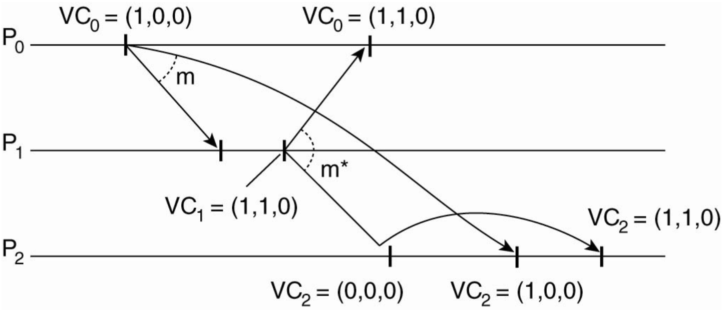
Example

- Violation: If \(P_1\) sends a message requiring \(VC=(1,1,0)\) but \(P_2\) only has \((0,0,0)\), \(P_2\) must wait. It effectively says "This message depends on an update from \(P_0\) that I haven't seen yet".
| Feature | Totally Ordered Multicast | Causally Ordered Multicast |
|---|---|---|
| Ordering Rule | Every node processes all messages in the exact same sequence, regardless of relationship. | Only messages with a causal relationship (\(A \to B\)) must be ordered. Concurrent messages ($A |
| Primary Goal | Global Consistency: Ensure every replica transitions through identical states (e.g., replicated database). | Causal Integrity: Ensure replies never appear before the original message (e.g., social media comments). |
| Logical Clock Used | Lamport Timestamps (Total Order via \(L.i\) tie-breaking). | Vector Clocks (Partial Order via \(N\)-dimensional arrays). |
| Concurrency Handling | Forces concurrent events into an arbitrary but identical total order. | Allows concurrent events to be processed in any order, improving performance. |
| Blocking/Waiting | High: A node must wait for Acks from everyone to ensure no "earlier" message exists. | Lower: A node only waits if the Vector Clock shows it is missing a causal predecessor. |
| Acknowledgment (Ack) Requirement | Mandatory: Every node must broadcast an Ack to move the global "time" forward for the group. | Not Required for Ordering: The Vector Clock carries all necessary metadata to verify causality. |
| Bottleneck Risk | One slow node can freeze the entire system (the "slowest member" problem). | Much more resilient; only nodes involved in a specific causal chain are affected by delays. |
| Scalability | Poor: \(O(n^2)\) messages per broadcast due to the global Ack requirement. | Better: Avoids global synchronization for unrelated messages. |
In a distributed system, "Concurrent" doesn't mean the messages don't reach everyone; it means the messages were sent without any knowledge of each other.
The system embraces concurrency. If Message A and Message B are unrelated, the system doesn't care which one you process first.
- Result: Node 3 might process A then B, while Node 4 processes B then A. This is perfectly allowed because there is no "causal" reason to force one to wait for the other. This makes the system much faster!
- Everyone eventually receives every message.