Analyzing Graphs

Graph Theory & Data Structures

Fundamentals

• Definition: A graph \(G = (V, E)\) consists of a set of Vertices (Nodes) and a set of Edges (Links).
• Types:
  • Directed: An edge \((u, v)\) goes from \(u\) to \(v\) but implies nothing about the return path.
  • Undirected: An edge \((u, v)\) implies \((v, u)\) automatically.
  • Weighted: Edges can carry numerical labels (weights).
• Terminology:
  • Out-Neighbor: If edge \((u, v)\) exists, \(v\) is an out-neighbor of \(u\), and \(u\) is an in-neighbor of \(v\).
  • In-Degree / Out-Degree: The count of edges entering or leaving a specific vertex.
• Sparsity: Most real-world graphs (Social Networks, The Web, Roadways) are sparse. The number of edges is typically closer to \(|V|\) than to the maximum possible \(|V|^2\).

Graph Representations

Adjacency Matrix

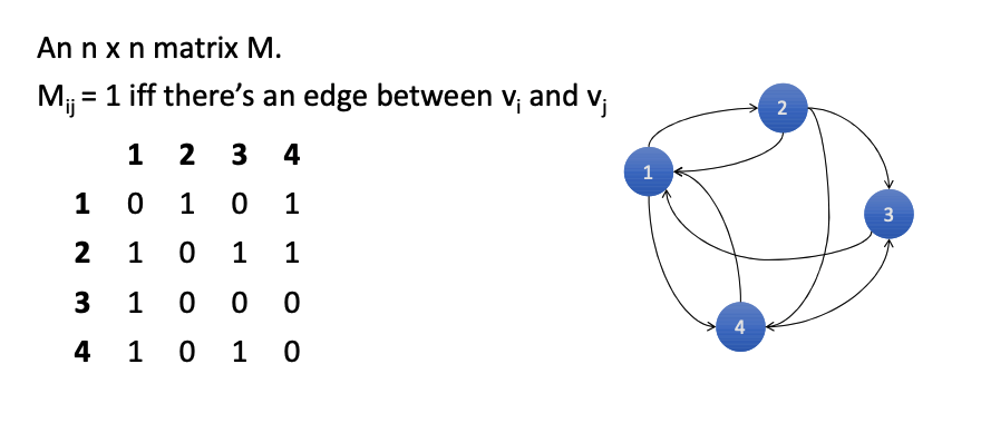
An \(N \times N\) matrix where \(M_{ij} = 1\) if an edge exists between \(v_i\) and \(v_j\).

• Structure: A dense grid representing all possible connections.
• Pros:
  • Excellent for mathematical operations (Matrix Multiplication).
  • Fast neighborhood checks (\(O(1)\) lookup).
  • Optimized for GPUs (CUDA loves matrices).
• Cons:
  • Wasted Space: For sparse graphs, the matrix is almost entirely zeros.
  • Slow Iteration: Finding neighbors takes \(O(N)\) because you must scan the whole row, even if there is only 1 neighbor.

Adjacency List

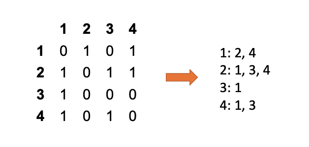
An array (or map) where row \(i\) contains a list of only the out-neighbors of vertex \(v_i\).

• Structure: Conceptually similar to a Postings List in search indices.
• Pros:
  • Compact: Much smaller than a matrix for sparse graphs.
  • Fast Traversal: Finding out-neighbors is efficient because they are directly stored.
• Cons:
  • Hard to find In-Neighbors: You cannot easily see "who points to me" without searching every other list (or building a second reverse-graph list).

Edge List

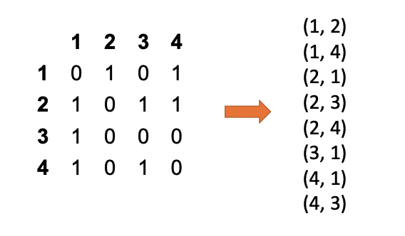
A simple flat list of pairs representing edges (e.g., (1, 2), (1, 4), (2, 1)).

• Structure: Just a collection of "from-to" tuples.
• Pros:
  • Extremely simple to create (just append new edges).
  • Ideal for initial data ingestion.
• Cons:
  • Hard to Query: Finding neighbors requires scanning the entire list. It is generally not used for processing, but rather as an intermediate format.
  • Life Hack: You can convert an Edge List into an Adjacency List using a groupByKey operation.

Graph Algorithms & Scale

Common Graph Problems

Graph theory maps directly to real-world engineering challenges:

• Shortest Path: Google Maps, Logistics.
• Minimum Spanning Tree (MST) & Min-Cut: Utility line planning, Disease spread modeling.
• Max-Flow: Airline scheduling.
• Graph Coloring: Scheduling final exams (avoiding collisions).
• Bi-Partite Matching: Dating sites (matching Set A to Set B).

The Web Graph Structure

• Scale: The web is massive, with ~50 billion pages (vertices) and ~1 trillion links (edges).
• Power Law: It follows a strict power law distribution (\(P(k) \sim k^{-\gamma}\)). Most pages have very few links (0 or 1), while a tiny fraction have millions. This "Long Tail" makes processing difficult.
• "Dark Web": In this context, it simply refers to pages not indexed by search engines (e.g., behind logins), not necessarily illegal content.
• Big Data Definition: For graphs, even 60GB is considered "Big Data" because the complexity of traversing edges makes it computationally heavy, necessitating tools like Hadoop or Spark.

Parallel Graph Processing

• The Paradigm: Most parallel graph algorithms consist of two steps:
  1. Local Computation: Calculating a value for a node based on its current state (Independent).
  2. Propagation: Sending that value to neighbors (Graph Traversal).
• Best Representation: Adjacency Lists are the superior format here. They map naturally to MapReduce Key-Value Pairs (Key = Vertex, Value = Neighbor List).
• Execution: "Propagation" is effectively a Shuffle/Reduce operation, where messages are grouped by destination vertex.

Single-Source Shortest Path (SSSP)

• The Problem: Find the shortest path from a single source node to all other nodes in the graph.
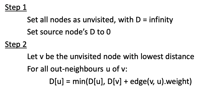
• Sequential Solution (Dijkstra): The standard algorithm uses a global priority queue to visit the "unvisited node with the lowest distance" (\(D\)) and relax its edges.

• MapReduce Failure: Dijkstra cannot be efficiently implemented on MapReduce.
  • Why? The step "Find node with Minimum \(D\)" requires global knowledge of the entire graph's state. It is not a local computation, breaking the parallelism.
• The Parallel Solution: Instead of Dijkstra, distributed systems use Parallel Breadth-First Search (pBFS).

The Challenge: Unweighted Graphs & Iteration

• Goal: Find the shortest path (fewest hops) from a source node to all other nodes.
• Inductive Logic:
  • \(dist(\text{source}) = 0\)
  • \(dist(v) = 1 + \min(dist(u))\) for all neighbors \(u\).

Hadoop MapReduce Implementation

Implementing this on MapReduce requires preserving the graph structure across stateless jobs.

Let keys be nodes \(n\), values be (\(d\) which is distance to \(n\), adjacency list of \(n\)),

Key: NodeID | Value: (Current_Distance, List_of_Neighbors)

• The Mapper:
  • Emits updated distances (\(d+1\)) to all neighbors (\(m\)). → \((m : d+1)\)
  • Crucially: Must also emit the original node structure \((n : d)\) so the adjacency list is not lost for the next iteration.
    • So when we say "Next Iteration," we mean an entirely new MapReduce process that starts up, reads the file created by the previous process, and runs the same logic again.
    • 1 Iteration = 1 MapReduce Job.
• The Reducer:
  • Receives multiple messages for a node ID: some are potential new distances (integers), and one is the Node object itself.
  • Updates the node's distance to the minimum of all received values.
• Iteration Cycle: Since MapReduce jobs terminate, we must chain them. Job 1 reads from HDFS and writes to HDFS; Job 2 reads Job 1's output. We repeat this until the graph "settles".

Algorithm Pseudocode

The following Python-like pseudocode describes the Parallel Breadth-First Search (pBFS) logic used to replace Dijkstra's algorithm.

# Mapper: Propagates distances and preserves structure
def map(id, node):
    emit(id, node)              # Pass the node structure to next generation
    for m in node.adjList:
        emit(m, node.d + 1)     # Send "d+1" reachability to neighbors

# Reducer: Finds the shortest path discovered so far
def reduce(id, values):
    d = infinity
    node = None

    for o in values:
        if isNode(o):           # Recover the Node object
            node = o
        else:                   # It's a distance message
            d = min(d, o)

    node.d = min(node.d, d)     # Update with shortest distance found
    emit(id, node)

The implementation of Single-Source Shortest Path (SSSP) on MapReduce requires a specific Node object structure containing both the distance from the source (d) and the list of out-neighbors (adjList) to preserve graph topology between stateless jobs. Because the Reducer receives a mix of data types—both the simple distance values sent by neighbors and the complex Node objects themselves—you must use ObjectWritable and reflection to dynamically distinguish between them at runtime. Additionally, a critical optimization: adding a last_updated field to the Node object so that Mappers only propagate messages if the node's distance actually changed in the previous iteration, thereby reducing unnecessary network traffic.

Because MapReduce is completely stateless, it has "amnesia" between jobs; it can’t just remember the graph in memory for the next loop like a normal program would. So, for every single iteration of our algorithm, we are forced to write the entire graph—including those massive adjacency lists that aren't even changing—all the way down to the slow HDFS hard drive, only to immediately read them back up again for the next round. It is a massive waste of I/O and time, which is exactly why newer tools like Spark were invented to keep data in memory, but in the strict MapReduce world, this expensive "disk-and-back" cycle is the unavoidable penalty we pay for iteration.

Optimization & Termination

• Path Reconstruction: The basic algorithm only calculates distance. To reconstruct the actual path, the Node object must store a previous field (the ID of the node that provided the shortest distance).
• Termination: We know when to stop iterating when a full job completes with zero updates to any node's distance (the graph has converged).

• Performance Reality:

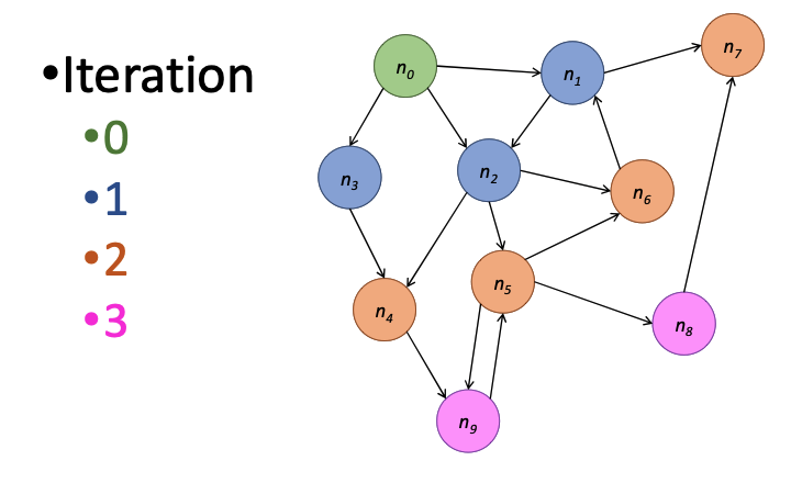
  • Kevin Bacon Number: Real-world graphs (like social networks) often have small diameters (~6 hops), so the number of iterations is manageable.
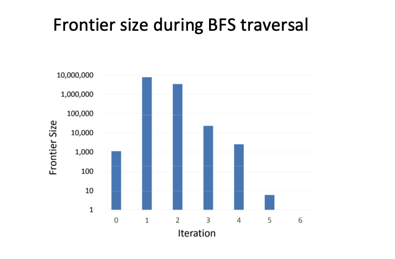
  • Frontier Size: The number of active nodes (frontier) grows rapidly then shrinks, varying based on the link distribution.
    • "Active Nodes" (the Frontier) are only the nodes that changed their distance in the previous round.

  

  Here is the reality check on whether this algorithm actually finishes before the heat death of the universe. The good news is that real-world graphs—like social networks or the web—exhibit the "Small World" property, meaning the diameter is surprisingly small (often around 6 hops, like the Kevin Bacon number), so we typically only need to chain about 6 or 7 MapReduce jobs to traverse the whole thing, which is entirely manageable. However, you need to watch out for the "Frontier"—that is the set of nodes active in any given iteration; it doesn't grow linearly, but rather explodes outward in the middle iterations before dying down, meaning your cluster will face a massive spike in workload halfway through the process before idling down at the end.

Code Adaptation for Weighted Edges

To support weighted graphs, the algorithm structure remains largely identical to the unweighted version. The only critical change occurs in the Mapper, where the distance calculation now uses the specific edge weight (m.w) instead of a constant 1.

# Mapper: Now adds specific edge weights
def map(id, node):
    emit(id, node)                # Pass structure forward
    for m in node.adjList:
        # KEY CHANGE: Use m.w (weight) instead of +1
        emit(m.id, node.d + m.w)

# Reducer: Logic remains exactly the same
def reduce(id, values):
    d = infinity
    node = None
    for o in values:
        if isNode(o):
            node = o
        else:
            d = min(d, o)         # Still just finding the minimum

    node.d = min(node.d, d)
    emit(id, node)

Termination Complexity (The "Fuzzy Frontier")

• Re-visiting Nodes: Unlike unweighted BFS where a node is visited once and "done," weighted graphs allow a node to be updated multiple times if a "longer path with lighter weights" is found later. This creates a "Fuzzy Frontier".
• Iteration Count: The number of iterations is no longer determined by the graph's diameter (hops). Instead, it depends on the length of the longest cycle-free path, which can be significantly larger, potentially requiring many more MapReduce jobs. For unweighted, the # of iterations needed is the length of the longest “shortest path” (usually short).

Parallel BFS vs. Dijkstra

• Dijkstra's Limitation: Dijkstra efficiently investigates only the "lowest-cost" node using a global priority queue. This requires Global State, which does not exist in MapReduce.
• The MapReduce Compromise: We are forced to use Parallel BFS, which blindly investigates all active paths in parallel. It is less efficient (investigates more nodes) but is the only way to operate without shared memory.

Note

The above concepts seem a bit confusing to me… I asked Gemini to generate a sample program for me:

// --- STEP 1: INITIALIZATION ---
// We start by creating the initial state of the graph.
// This is done BEFORE the loop starts.
var currentGraph = graph.map { case (id, (dist, neighbors)) =>
  // Check: Is this the specific Start Node we are searching from?
  if (id == startNodeID) {
    // Yes: Set distance to 0 (Source)
    // Structure: (NodeID, (Distance=0, [List of Neighbors]))
    (id, (0, neighbors))
  } else {
    // No: Set distance to "Infinity" (Int.MaxValue)
    // We haven't found a path to this node yet.
    (id, (Int.MaxValue, neighbors))
  }
}

var iterationCount = 0
var updatesMade = 0L // Tracks how many nodes changed distance in this round

// --- STEP 2: THE ITERATION LOOP (The "Job Chain") ---
// This loop replaces the manual "Job 1 -> Job 2 -> Job 3" chaining in Hadoop.
do {
  iterationCount += 1

  // ============================================================
  // THE MAPPER PHASE (flatMap)
  // Corresponds to the Mapper in Slide image_20db61.png
  // ============================================================
  val messages = currentGraph.flatMap { case (id, (currentDist, neighbors)) =>

    // ----------------------------------------------------------
    // JOB A: SELF PRESERVATION (Topology)
    // Slide Reference: "emit(id, node)"
    // ----------------------------------------------------------
    // We must emit the node AS-IS. If we don't, the Reducer will receive
    // distance updates but won't know who the neighbors are for the NEXT round.
    // The node would effectively lose its edges and become a dead end.
    val selfPreservation = Seq((id, (currentDist, neighbors)))

    // ----------------------------------------------------------
    // JOB B: PROPAGATION (Shouting to Neighbors)
    // Slide Reference: "for m in adjList: emit(m, node.d + 1)"
    // ----------------------------------------------------------
    // We only send messages if we have actually been visited (dist < Infinity).
    val neighborMessages = if (currentDist < Int.MaxValue) {
      neighbors.map(neighborID => {
        // Create a message for the neighbor "m".
        // Key: neighborID (so it routes to the right place)
        // Value: (New Distance Proposal, Empty List)
        // Note: The list is empty because we don't know the neighbor's friends!
        (neighborID, (currentDist + 1, List.empty[Int]))
      })
    } else {
      // If we haven't been visited yet, we stay silent.
      Seq.empty
    }

    // Combine both sets of messages into one big stream.
    // Spark will now shuffle these messages across the network so that
    // all messages for "Node X" end up on the same machine.
    selfPreservation ++ neighborMessages
  }

  // ============================================================
  // THE REDUCER PHASE (reduceByKey)
  // Corresponds to the Reducer in Slide image_20db61.png
  // ============================================================
  val newGraph = messages.reduceByKey { (messageA, messageB) =>
    // This function runs whenever two messages land on the same Node ID.
    // We need to merge them into one best result.

    // 1. RECOVER STRUCTURE
    // One of these messages is the "Self Preservation" message containing the
    // real neighbor list. The others are just "Distance Proposals" with empty lists.
    // We check which one has data and keep it.
    // Slide Reference: "if isNode(o): node = o"
    val neighbors = if (messageA._2.nonEmpty) messageA._2 else messageB._2

    // 2. MINIMIZE DISTANCE
    // Compare the distances and keep the smallest one.
    // Example: messageA might say "Distance 5", messageB might say "Distance 3".
    // Slide Reference: "d = min(d, o)"
    val minDist = math.min(messageA._1, messageB._1)

    // Return the merged result: Best Distance + The Neighbor List
    (minDist, neighbors)
  }

  // ============================================================
  // THE CHECK (Counting Changes)
  // Corresponds to "Quitting Time" in Slide image_20db85.jpg
  // ============================================================
  // We join the New Graph with the Old Graph to see who actually changed.
  // This triggers the "Action" that forces Spark to actually run the job.
  val changes = newGraph.join(currentGraph).filter {
    case (id, ((newDist, _), (oldDist, _))) =>
      // A change only counts if we found a SHORTER path.
      newDist < oldDist
  }.count()

  // Update our state for the next loop
  updatesMade = changes
  currentGraph = newGraph

  println(s"Iteration $iterationCount: Updated $updatesMade nodes.")

// Continue looping as long as we are still making updates (The Frontier > 0).
} while (updatesMade > 0)

Issues with MapReduce and Introduction to PageRank

MapReduce Iteration vs. Spark

• MapReduce Bottlenecks:
  • Disk I/O Overhead: In iterative MapReduce algorithms, everything is written to the HDFS (Hard Disk) at the end of an iteration and then loaded again for the next, causing significant latency.
  • Network Overhead: The entire graph structure must be sent to the reducers during each iteration, only to have them send it back, wasting bandwidth.
• Spark Optimization:
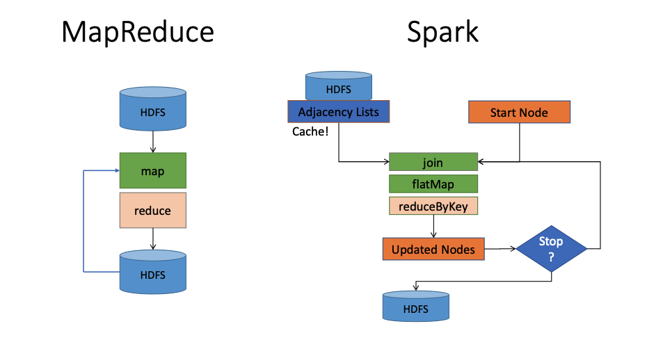
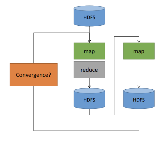
  • Architecture Comparison:
    • MapReduce Flow: Data flows strictly from HDFS \(\rightarrow\) Map \(\rightarrow\) Reduce \(\rightarrow\) HDFS.
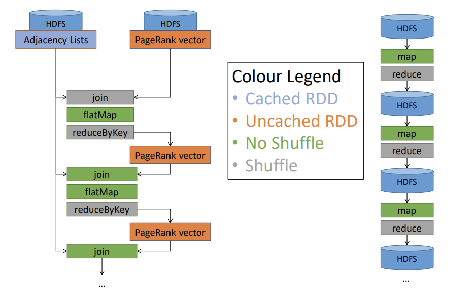
    • Spark Flow: Data is loaded from HDFS into memory (Cache). Operations like join, flatMap, and reduceByKey occur in a loop (iteration) directly on the cached data before writing the final result to HDFS.
      • Diagram below showing a complex flow: Data loads from HDFS into 'Adjacency Lists' which are cached. A loop performs transformations (Join -> FlatMap -> ReduceByKey) to update nodes. A decision diamond 'Stop?' determines if the loop continues or if data is written to HDFS.
  • Transformation Types:
    • Narrow Dependencies (Green): Local transformations that require no shuffles (e.g., map, flatmap).
    • Wide Dependencies (Orange): Reduce-like transformations that require shuffles (data movement across the network), such as reduceByKey.

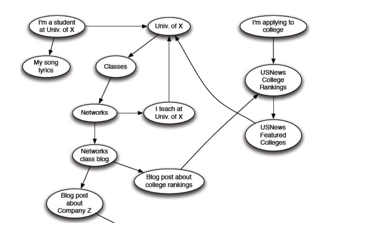
The Web as a Directed Graph

• Graph Structure: The web is modeled as a directed graph where Nodes represent web pages (e.g., "I'm a student at Univ of X") and Edges represent hyperlinks (e.g., pointing to "Classes" or "Networks").

• The Trust Challenge:
  • Ambiguity: A query like "University of Waterloo" returns multiple results. A fake site (fakeuw.ca) might look identical to the real site (uwaterloo.ca) in terms of content/keywords.
  • Failure of Ranked Retrieval: Standard information retrieval techniques based on content matching fail to distinguish between the authoritative source and the imposter.
• The Solution (Link Analysis): To determine "Who to trust," we rely on the link structure. The core trick is that trustworthy pages tend to point to each other.

PageRank: Formulation and Solution

PageRank: The "Flow" Formulation

• Ranking Concept: Not all web pages are equally "important." For example, www.stanford.edu is inherently more significant than a random personal blog www.joeschmoe.com. We rank pages based on the diversity and connectivity of the web-graph link structure.
• Links as Votes:
  • Basic Idea: A link from Page A to Page B is considered a "vote" for Page B.
  • Metric: A page is considered more important if it has more in-links (incoming edges).
• Recursive Definition: Not all votes are equal.
  • Links from important pages count more than links from unimportant pages.
  • This creates a recursive question: To know a page's importance, you need to know the importance of the pages linking to it.
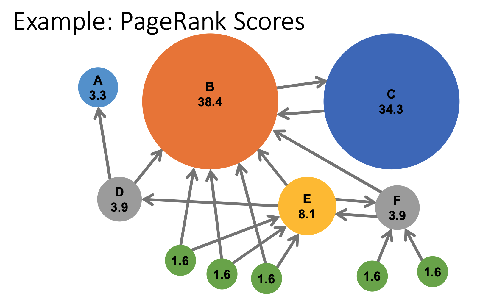
• Visualizing Scores: In a calculated PageRank graph, nodes with many incoming links from other high-value nodes (like Node B with a score of 38.4 or Node C with 34.3) become the largest and most influential in the network.

Simple Recursive Formulation

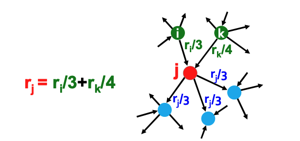
• The "Flow" Concept: PageRank assigns an importance score \(r_j\) to a page \(j\) based on the collective "votes" of the pages pointing to it.

  • Vote Weighting: Not all links are equal. A link from page \(i\) to page \(j\) is considered a vote proportional to the importance of the source page (\(r_i\)) divided by its number of outgoing links (\(d_i\)).

  • The Equation:

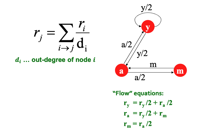
    \[ r_j = \sum_{i \to j} \frac{r_i}{d_i} \]

    Where \(d_i\) is the out-degree of node \(i\).

    

• System of Equations: For a graph with 3 nodes (\(y, a, m\)), we can derive a set of "flow equations" (e.g., \(r_y = r_y/2 + r_a/2\)).

Solving the Flow Equations

• The Problem: With 3 equations and 3 unknowns (and no constants), there is no unique solution. All solutions are equivalent modulo a scale factor.
• The Constraint: To enforce uniqueness, we add the constraint that the sum of all PageRanks must equal 1:

\[ r_y + r_a + r_m = 1 \]

• Methodology: While Gaussian elimination works for small examples (finding \(r_y = 2/5, r_a = 2/5, r_m = 1/5\)), it is inefficient for web-scale graphs, requiring a new formulation.

Matrix Formulation and Power Iteration

• Stochastic Adjacency Matrix (\(M\)): We can represent the link structure as a matrix where column \(i\) represents the outgoing links from page \(i\).
  • If page \(i\) points to \(j\), then \(M_{ji} = \frac{1}{d_i}\) (otherwise 0).
  • Property: This is a column stochastic matrix, meaning every column sums to 1.

• Power Iteration Algorithm: This is the practical method for solving PageRank on large graphs.

  1. Initialize: Set all ranks \(r_j = 1/N\).
  2. Iterate: Update the ranks using the equation:
  \[ r'_j = \sum_{i \to j} \frac{r_i}{d_i} \]
  1. Repeat: Set \(r = r'\) and repeat until convergence.

Random Walk Interpretation

• Concept: Imagine a "random web surfer" at page \(i\) at time \(t\). At time \(t+1\), the surfer follows an out-link uniformly at random.
  • Note: This does not simulate a literal person, but constructs a probability distribution of where a random walker might be.

• Stationary Distribution:

  • We define a vector \(p(t)\) where the \(i^{th}\) coordinate is the probability that the surfer is at page \(i\) at time \(t\).
  • The movement is defined by:
  \[ p(t+1) = M \cdot p(t) \]

  • The Stationary Distribution is reached when the probability distribution stops changing:

    \[ M \cdot p(t) = p(t) \]

    In this state, \(p(t)\) represents the final PageRank scores.

• Existence and Uniqueness: According to Markov process theory, a unique stationary distribution exists if the graph is Ergodic. To be ergodic, the graph must be:

  1. Connected: Not comprised of disjoint components.
  2. Not Bi-partite: The structure cannot simply oscillate back and forth between two distinct sets of nodes.

PageRank: The Google Formulation

Convergence Questions

When iterating the PageRank algorithm, we face three critical questions regarding stability:

1. Does it converge? (Do the numbers stop changing?)
2. Does it converge to what we want? (Is the result useful?)
3. Are the results reasonable?

The Convergence Problem (Oscillation)

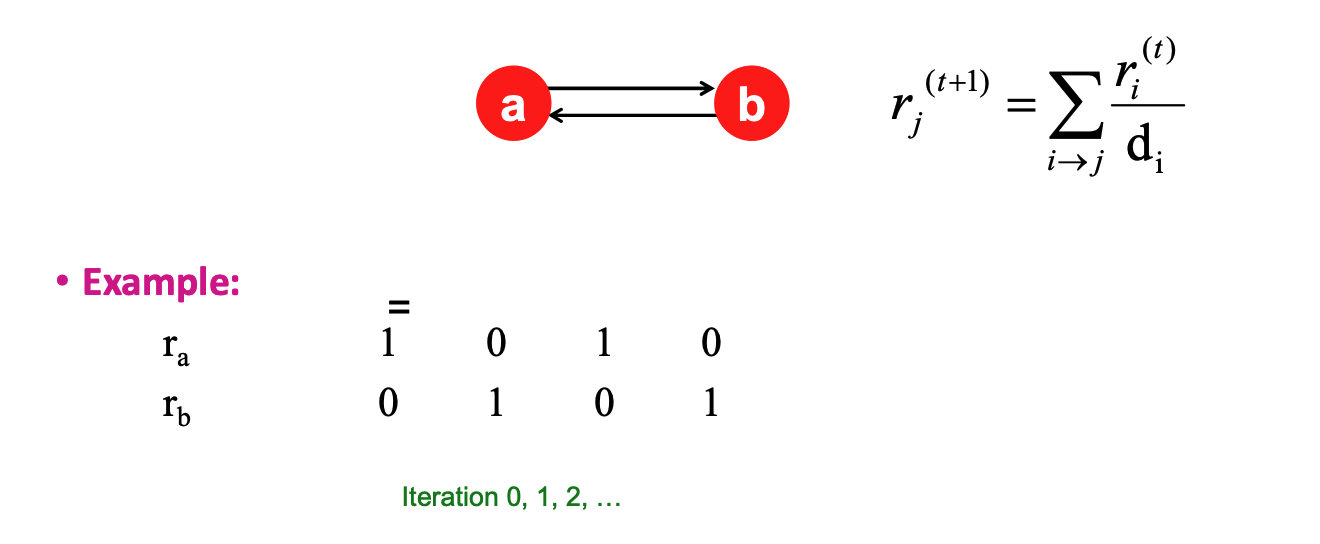
• Issue: In certain graph structures, such as a bi-partite graph (e.g., two nodes pointing only at each other: \(a \leftrightarrow b\)), the scores never settle. They oscillate (vacillate) indefinitely between values (e.g., 1,0 \(\rightarrow\) 0,1 \(\rightarrow\) 1,0).

• Requirement: For a stationary distribution to exist, the graph must be connected and vertex aperiodic.
  1. The Graph Must Be Connected
     • Definition: The graph cannot be broken into separate, isolated islands. There must be a path that allows the "random surfer" to eventually reach any part of the graph from any other part. Why it matters: If the graph is disconnected (e.g., two distinct groups of websites that never link to each other), the random surfer would get stuck in whichever section they started in.
     • Consequence: The final scores (stationary distribution) would depend entirely on where the surfer started, meaning there is no single, unique "true" answer.
  2. The Graph Must Be Vertex Aperiodic
     • Definition: The random surfer must not get trapped in a predictable, rhythmic cycle.
     • The Math Rule (GCD): For every vertex \(v\), if you look at the lengths of all possible loops/cycles that start and end at \(v\), the Greatest Common Divisor (GCD) of those lengths must be 1.
       • Example of Failure (Bipartite Graph): Imagine two nodes pointing only at each other (\(A \leftrightarrow B\)).
         • To leave \(A\) and come back, you can take 2 steps (\(A \to B \to A\)), 4 steps, 6 steps, etc.
         • The GCD of \(\{2, 4, 6, ...\}\) is 2. Since \(2 \neq 1\), this graph is periodic.
     • Why it matters: In a periodic graph, the surfer oscillates back and forth forever (e.g., always at Node A on even steps, always at Node B on odd steps). The probabilities never settle down to a single steady value. A GCD of 1 ensures the walker's position becomes truly random over time.

Two Major Pathologies: Dead Ends and Spider Traps

The web is full of structures that break the basic PageRank math.

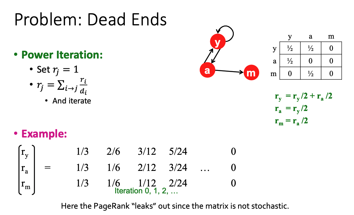
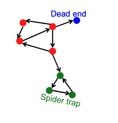
Dead Ends ("Leakage")

• Definition: Pages that have no out-links.
• Consequence: The random walker arrives at the page and has "nowhere to go."
• Mathematical Failure: The adjacency matrix column for this node sums to 0 instead of 1 (it is not stochastic). In the power iteration, importance "leaks out" of the system at every step until all PageRank scores eventually drop to zero.

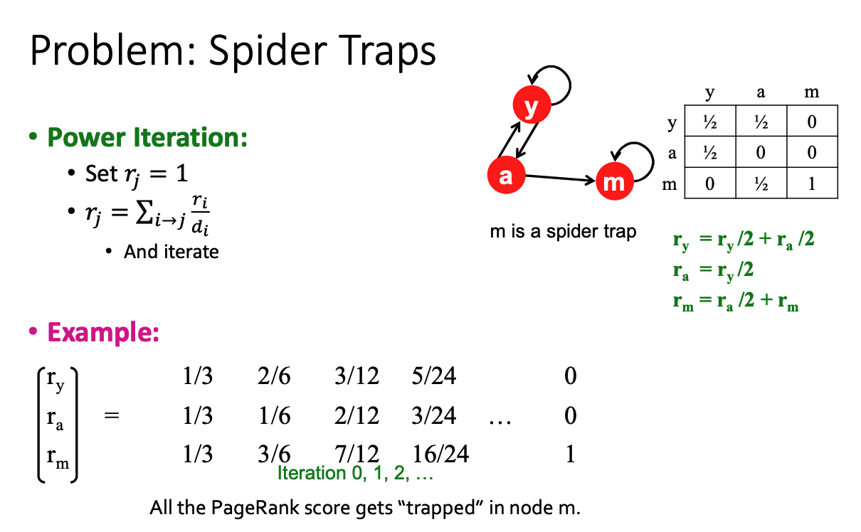
Spider Traps ("Absorption")

• Definition: A group of nodes (or a single node) where all out-links point within the group. There is no path out.
• Consequence: Once the random walker enters the trap, they cannot leave. They get "stuck" cycling within the trap.
• Mathematical Failure: The trap acts as a sink, eventually absorbing all the importance in the entire graph. The trap nodes get a score of 1, and everyone else gets 0.

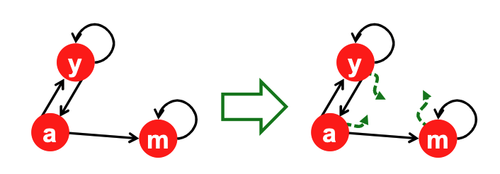
The Solution: Teleportation

To solve these issues, Google modifies the "Random Surfer" model to include teleportation (jumping to a random page).

Handling Spider Traps (The Damping Factor \(\beta\))

• Mechanism: At each time step, the random surfer has two options:
  1. Follow a Link: With probability \(\beta\) (typically 0.8 to 0.9), follow a real link at random.
  2. Teleport: With probability \(1-\beta\), jump to a random page anywhere in the graph.
• Result: The surfer will eventually "teleport out" of the spider trap, preventing it from absorbing all rank.

Handling Dead Ends (Matrix Adjustment)

• Mechanism: If a node is a dead end (no out-links), the surfer cannot choose option 1 (Follow an existing out-link on the page). Therefore, they always teleport (probability 1.0).
• Matrix Fix: To make the math work, we adjust the matrix column for the dead-end node. We replace the column of zeros with uniform probabilities (\(1/N\)), effectively saying, "If you hit a dead end, restart comfortably at a random page".

Why Teleports Solve the Problem

• Spider Traps:
  • Issue: Spider traps are not a mathematical error, but they ruin the utility of the results because they absorb all the importance rank.
  • Solution: Teleporting ensures the random surfer never gets stuck indefinitely; they will eventually teleport out of the trap in a finite number of steps.
• Dead Ends:
  • Issue: These are a mathematical failure because the matrix column is not stochastic (sums to 0), causing our initial assumptions to fail.
  • Solution: We force the matrix to be column-stochastic by making the surfer always teleport when they hit a dead end (nowhere else to go).

Solution: Random Teleports

• The "Google Solution":
  • At every single step, the random surfer has two distinct options:
    1. Follow a Link: With probability \(\beta\), follow an existing outbound link.
    2. Jump: With probability \(1-\beta\), jump to a random page anywhere in the graph.
• The conceptual model translates into the following formal equation:

\[ r_j = \underbrace{\sum_{i \to j} \beta \frac{r_i}{d_i}}_{\text{Link Part}} + \underbrace{(1 - \beta)\frac{1}{N}}_{\text{Teleport Part}} \]

• Variable Explanation:
  • \(r_j\): The PageRank score of the destination page \(j\).
  • \(\beta\): The damping factor (probability of following a link).
  • \(\sum_{i \to j}\): The summation of "votes" from all pages \(i\) that link to page \(j\).
  • \(r_i\): The current PageRank score of the source page \(i\).
  • \(d_i\): The out-degree of node \(i\) (the total number of links on page \(i\)).
  • \(N\): The total number of nodes (pages) in the graph.
• Logic Breakdown:
  1. The Link Contribution (\(\beta \frac{r_i}{d_i}\)): This part represents the flow of importance along the graph's edges. A page \(i\) passes its importance \(r_i\) to its neighbors, split equally among its \(d_i\) links. This flow is dampened by \(\beta\).
  2. The Teleport Contribution (\((1 - \beta)\frac{1}{N}\)): This part represents the random jumps. Since the surfer jumps to any page with equal probability (\(1/N\)), every page in the graph receives this tiny base amount of score, regardless of incoming links.
     • Note: This formulation assumes the matrix \(M\) has no dead ends. Dead ends must be removed during preprocessing or explicitly handled by setting their jump probability to 1.0.

The Matrix Method

Let

\[ A = \beta \cdot M + (1 - \beta) \cdot \left[ \frac{1}{N} \right] \]

The algorithm is defined as:

\[ \vec{r}_{new} = A \times \vec{r}_{old} \]

Convergence (The End Goal):

Eventually, multiplying by Matrix A stops changing the numbers.

PageRank with MapReduce

Simplified Approach (No Teleports)

• Concept: To understand the flow, we first implement a simplified version that ignores random jumps (teleportation) and dead-ends.
• Map Phase (Distribution):
  • The goal is for each node to "send" its current importance (rank) to its outgoing links.
  • Key Action: The mapper processes a node, calculates the share of rank each neighbor receives (current_rank / out_degree), and emits this share to the target neighbors.
  • Structure Preservation: Crucially, the mapper must also emit the node object itself (id, n) so that the graph structure (adjacency list) is passed to the reducer for the next iteration.
• Reduce Phase (Aggregation):
  • The goal is for each node to calculate its new importance based on incoming traffic.
  • Key Action: The reducer receives a list of messages for a given Node ID. Some messages are the Node object (from self), and others are rank values (votes from other nodes). It sums the rank values to update the node's n.rank.

Pseudocode Implementation

The following pseudocode illustrates the MapReduce logic. Note the distinction between emitting the node itself (to save state) and emitting rank values (to propagate influence).

def map(id, n):
    # 1. Pass the graph structure to the reducer
    emit(id, n)

    # 2. Calculate rank share for neighbors
    # p is the rank divided by out-degree (len(n.adj))
    p = n.rank / len(n.adj)

    # 3. Send rank share to each neighbor
    for m in n.adj:
        emit(m, p)

def reduce(id, msgs):
    n = None
    sum = 0

    # Process all incoming messages for this node ID
    for o in msgs:
        # If 'o' is the Node object, we save it (recovering structure)
        if o is Node:
            n = o
        # If 'o' is a number, it is a rank vote
        else:
            sum += o

    # Update the node's rank with the new sum
    n.rank = sum
    emit(id, n)

Comparison: PageRank vs. BFS

PageRank shares a structural similarity with Breadth-First Search (BFS) in MapReduce. Both belong to a class of graph algorithms that involve local computations at a node followed by propagating results (traversing) to neighbors.

• PageRank:
  • Map Output: Emits \(PR/N\) (Rank Share).
    • PR: Is the node's current importance score (n.rank).
    • N: Is the Number of Outgoing Links (or neighbors) that the node has (len(n.adj)).
  • Reduce Action: Calculates sum (Total Probability).
• BFS:
  • Map Output: Emits \(d+1\) (Distance + 1).
  • Reduce Action: Calculates min (Shortest Path).

Complete PageRank (Adding Teleports)

The simplified version is missing the "Random Jumps" (damping factor \(\beta\)) and handling for Dead Ends.

• Random Jumps Logic: Every node has a \(1 - \beta\) probability of "boredom," where the surfer jumps to any random page in the graph (probability \(1/N\)).
• Implementation Strategy: This modification handles the "taxation" logic where rank is constantly redistributed.
  • Location of Change: We only need to change the Reducer side. The Mapper continues to distribute the flow along edges, but the Reducer adds the base probability of the random jump when calculating the final sum.

The Code Implementation

The reducer is updated to explicitly handle the damping factor (\(\beta\)) and the random jump probability.

def reduce(id, msgs):
    n = None
    sum = 0
    for o in msgs:
        # 1. Recover Graph Structure
        # We find the Node object to preserve edges for the next round
        if o is Node:
            n = o
        # 2. Accumulate Votes
        # Sum up the rank shares received from neighbors
        else:
            sum += o

    # 3. Apply the PageRank Equation
    # sum * beta: The share from links
    # (1 - beta) / N: The share from global teleportation
    n.rank = sum * beta + (1 - beta) / N
    emit(id, n)

The Logic: Why \((1-\beta)/N\)?

• Global Contribution: In the random surfer model, every node contributes a fraction \((1 - \beta)\) of its current rank to a global "teleport pool" that is distributed to everyone else.
• Total Energy: Since the sum of all PageRank scores in the graph is always equal to 1, the total amount of rank being teleported across the entire network at any step is exactly equal to \((1 - \beta)\).
• Even Distribution: This total teleport energy is split evenly among all \(N\) nodes in the graph. Therefore, instead of sending \(N\) individual messages, we can mathematically calculate that every node receives exactly \((1 - \beta) / N\) rank from the global teleportation process.

Why the sum of all PageRank scores in the graph is always equal to 1?

\[ \begin{align*} \text{Total Sum} &= \sum_{j=1}^{N} r_j^{\text{new}} \\ &= \sum_{j=1}^{N} \left( \underbrace{\sum_{i \to j} \beta \frac{r_i}{d_i}}_{\text{Link Inflow}} + \underbrace{\frac{1-\beta}{N}}_{\text{Teleport Inflow}} \right) \\ &= \sum_{j=1}^{N} \sum_{i \to j} \beta \frac{r_i}{d_i} + \sum_{j=1}^{N} \frac{1-\beta}{N} \\ &= \underbrace{\sum_{i=1}^{N} \sum_{j \leftarrow i} \beta \frac{r_i}{d_i}}_{\text{Group by Sender } i} + \underbrace{N \cdot \frac{1-\beta}{N}}_{\text{Sum of Constant}} \\ &= \sum_{i=1}^{N} \beta \frac{r_i}{d_i} \cdot \underbrace{d_i}_{\text{Out-degree}} + (1 - \beta) \\ &= \sum_{i=1}^{N} \beta r_i + (1 - \beta) \\ &= \beta \underbrace{\sum_{i=1}^{N} r_i}_{=1 \text{ (Assumption)}} + (1 - \beta) \\ &= \beta(1) + 1 - \beta \\ &= 1 \end{align*} \]

The Link Sum (The Tricky Part)

\[ \sum_{j=1}^{N} \sum_{i \to j} \beta \frac{r_i^{old}}{d_i} \]

This looks messy, but think about what it represents physically.

• Perspective 1 (Receiver \(j\)): "I sum up everything I get from my neighbors."
• Perspective 2 (Sender \(i\)): "I send my rank out to my neighbors."

If we swap the summation order (sum over senders \(i\) instead of receivers \(j\)), we see that every node \(i\) pushes out exactly \(\beta \cdot r_i^{old}\) in total, split among its \(d_i\) children.

Advanced PageRank Implementation Details

Handling Dead-Ends

Dead-ends (nodes with no out-links) are problematic because they cause importance (rank mass) to leak out of the system.

• The Bad Approach (Option 1): Replacing dead-ends with links to every other node in the graph is a terrible idea because it turns a degree-0 node into a degree-N node, breaking the fundamental assumption that the graph is strictly sparse.
• The Post-Processing Approach (Option 2): A better method is to mathematically redistribute the "missing mass". First, calculate the sum of all current ranks (\(R\)). The missing mass is \(1 - R\), which represents the rank absorbed by dead ends. Finally, add \((1 - R) / N\) to all nodes.

• Implementation Tricks: In Spark, this can be tracked using a double accumulator. In MapReduce, you can use a "side-unloading" technique where reducers write out their portion of \(R\) to small files for the driver to load. This post-processing map step can be cleanly folded into the map phase of the next iteration to save time.
• The "Everyone" Key Alternative: Another approach is having dead-ends send their entire rank to a special key called "everyone". The reducer then takes the total mass accumulated at this key and adds \((1/N) \times \text{mass}\) to every node's sum. To prevent a massive bottleneck of messages, this requires an In-Memory Combiner (IMC) so each mapper only sends one "everyone" message per reducer.

Numerical Stability and Log Masses

In a graph with billions of nodes, the individual PageRank values become microscopically small, highlighting limitations in standard floating-point representations.

• The Solution: We store the natural logarithms of the ranks instead of the raw probabilities.
• Math Operations: Multiplication turns into simple addition: \(m \times n \to a + b\) (where \(a = \ln m\) and \(b = \ln n\)).
  • Addition (\(m + n\)) becomes a piecewise function evaluating \(b + \ln(1 + e^{a-b})\) or \(a + \ln(1 + e^{b-a})\) depending on whether \(a < b\) or \(a \ge b\).
• The Real Reason: While a standard double actually has enough bits to avoid underflow for these small numbers, using log probabilities prevents severe rounding errors. It makes operations mathematically stable when adding incredibly small numbers to relatively large numbers.

Transitioning from MapReduce to Spark

MapReduce is highly inefficient for iterative algorithms like PageRank.

• MapReduce Flaws: It pointlessly resends the static adjacency list data across the network every single iteration, performs needless shuffling and filesystem access, and incurs a long startup penalty for every new job in the iteration loop.
• The Spark Advantage: Spark caches the static Adjacency List (the graph structure) in memory as an RDD.
• Avoiding Shuffles: The iteration logic uses join, flatMap, and reduceByKey to merge the dynamic PageRank vector with the cached graph structure. By pre-partitioning both the adjacency list and the rank vector by node ID, Spark achieves "narrow dependencies" and completely eliminates the network shuffle for the joins.

• Performance: Because of these architectural improvements, Spark executes iterations much faster than MapReduce (e.g., 28 seconds vs. 80 seconds per iteration on a 60-machine cluster).

Spark PageRank Implementations

Apache Spark significantly reduces the verbosity of PageRank compared to MapReduce. While a MapReduce implementation in Bespin might take over 600 lines of code, Spark can express the same logic concisely.

The Spark implementations generally follow these steps:

1. Load URLs and initialize their neighbors.
2. Initialize the ranks to 1.0.
3. Iteratively calculate contributions by joining links with current ranks and distributing the rank evenly among out-links.
4. Re-calculate the new rank using the damping factor.

These basic examples assume there are no dead links in the graph and scale the total mass to \(N\) instead of 1.

PySpark Code Snippet:

# Calculates and updates URL ranks continuously using PageRank algorithm.
for iteration in range(iterations):
    # Calculates URL contributions to the rank of other URLs.
    contribs = links.join(ranks).flatMap(lambda url_urls_rank: computeContribs(
        url_urls_rank[1][0], url_urls_rank[1][1]
    ))
    # Re-calculates URL ranks based on neighbor contributions.
    ranks = contribs.reduceByKey(add).mapValues(lambda rank: rank * 0.85 + 0.15)

PageRank Improvements

Evolution of Search Ranking

Early search engine ranking relied heavily on Term Frequency and Document Frequency (TF and DF) alongside logarithms. This approach was highly vulnerable to Term Spam, where creators would hide repeated words or synonyms (e.g., in non-rendering HTML div tags) to manipulate search results.

To combat this, PageRank introduced a new philosophy: trust what others say about a page, not what the page says about itself. Search engines began using the link text (anchor text) and surrounding text from inbound links as search terms instead of relying solely on the page's own contents.

However, this solution introduced its own vulnerabilities. Coordinated efforts could manipulate the anchor text of inbound links to associate unrelated pages with specific terms, famously resulting in the biography of President George W. Bush ranking as the top result for the query "miserable failure".

Link Spamming and Farm Techniques

As PageRank became the standard, malicious actors developed new techniques to artificially inflate their rankings.

• Forum and Comment Spam: Spammers exploit high-ranking websites that allow user posting (like YouTube, Facebook, or news sites) by dropping links to their own webpages. Because the host site has a high PageRank, the spammer receives a portion of that high rank. Furthermore, the spammer dictates the link text, effectively choosing the search terms they want to rank for.
• Spam Farming: This technique leverages "spider traps" to hoard rank. While random jumps (teleportation) prevent a trap from accumulating all the rank in a network, the local topology can still heavily boost a target page.

In a spam farm, the page intended for promotion is set up with millions of hidden links pointing to internal "farm pages". These farm pages passively accumulate random-jump weight from the network and then link directly back to the target page, funneling all their accumulated rank back to artificially boost it.

The Mechanics of Link Spamming

To understand how to defeat link spam, we must analyze the web from the spammer's perspective, dividing it into three categories:

• Inaccessible Pages: Most of the internet, which the spammer cannot edit.
• Accessible Pages: External sites where the spammer can post links (e.g., forums) to inject rank into their trap.
• Owned Pages: The pages the spammer directly controls, consisting of the target page (\(t\)) and millions of dummy "farm pages" (\(M\)).
• The Trap: The spammer links the target page to millions of farm pages, and all farm pages link directly back to the target. This ensures any rank that enters the trap stays within it.

Mathematical Analysis of a Spam Farm

We can define the PageRank of the target page (\(y\)) and the farm pages (\(z\)) mathematically to understand why the trap is so effective.

• \(x\): total contribution of accessible pages to \(t\)
• \(y\): PageRank of \(t\) (boosted page)
• \(z\): PageRank of a single farm page

The rank of a single farm page is its share of the target page's rank plus the teleportation factor:

\[ z = \frac{\beta y}{M} + \frac{\alpha}{N} \]

The rank of the target page is the sum of external contributions, the rank from all farm pages, and the teleportation factor:

\[ y = x + M \beta z + \frac{\alpha}{N} \]

By substituting \(z\) into the equation for \(y\), we get:

\[ y = x + M \beta \left[ \frac{\beta y}{M} + \frac{\alpha}{N} \right] + \frac{\alpha}{N} \]

Ignoring the final very small \(\frac{\alpha}{N}\) term, this simplifies to the final target page rank:

\[ y = \frac{x}{1 - \beta^2} + \frac{\beta M}{(1 + \beta)N} \]

• Amplification: The \(\frac{x}{1 - \beta^2}\) term shows how the trap amplifies incoming links (e.g., \(3.6x\) amplification for \(\beta = 0.85\)).
• Linear Growth: The \(\frac{\beta M}{(1 + \beta)N}\) term proves the target page's rank grows linearly with the number of farm pages \(M\) (e.g., \(0.45 \frac{M}{N}\) for \(\beta = 0.85\)).

Initial (Flawed) Solutions

The first major attempt to stop link spam was the introduction of the nofollow attribute for links.

• The Concept: Convince forums and news sites to tag user-generated links as nofollow, instructing the search engine to ignore them for ranking purposes.
• The Failure: This successfully cuts off the rank injected from accessible pages (effectively making \(x = 0\) in the equation: \(y = \frac{x}{1-\beta^2} + \frac{\beta M}{(1+\beta)N}\)).
• The Loophole: However, because the target's rank is still directly proportional to \(M\), the spammer can still boost their rank arbitrarily high simply by generating more cheap dummy pages. Attempts to filter out small farm pages simply lead to spammers adding filler content to bypass the rules.

TrustRank (Personalized PageRank)

The definitive solution is modifying the PageRank algorithm to ensure random jumps (teleportation) do not land on farm pages, starving them of rank.

Seed Selection

• The system uses an "Oracle" (human curation) to collect a small set of highly trustworthy "seed pages".
• These are typically domains with strict entry requirements like .edu or .gov.

The Mechanism

• In Personalized PageRank, the algorithm only teleports to this curated trust set, meaning each trust page is initialized to 1 and the trust sums to a value \(M\) instead of 1.
• Because trustworthy pages mostly link to other trustworthy pages, and spam pages mostly link to other spam pages, this isolates the "good" partition of the web.
• After iterations, pages are assigned a trust factor between 0 and 1; a threshold is picked, and anything below it is marked as spam.

Trade-offs and Constraints

• Curating Costs: Human curation is expensive, so the seed set must be kept as small as possible.
• Trust Dilution: However, fewer seed pages mean less overall trust in the system. This forces a lower threshold, allowing more borderline spam pages to slip through.
• Link Distance: A page's final Trust score is roughly proportional to its link distance from a verified "good" seed page.

Seed Selection and Bootstrapping Trust

Selecting the initial "Oracles" or seed nodes for TrustRank is challenging. You cannot simply use the top pages by overall PageRank (as spam may have infiltrated the top ranks), and restricting seeds exclusively to .edu or .gov domains ignores many highly trustworthy commercial or organizational sites.

To combat the limitations of a small seed set, search engines use a Bootstrapping process to iteratively discover and verify new trustworthy pages:

1. Run standard PageRank.
2. Select the top pages and verify their trustworthiness to act as new seeds.
3. Run TrustRank using the expanded seed set.
4. Set a conservative threshold to avoid false positives, remove identified spam pages from the graph, and repeat the cycle.

Spam Mass Calculation

Instead of relying solely on a binary trust threshold, we can measure what fraction of a page's rank originates from untrusted sources. This metric is called Spam Mass.

• \(r_p\): The standard PageRank of page \(p\).
• \(r_p^+\): The PageRank of \(p\) calculated when random jumps only lead to Trusted seed pages.
• \(r_p^-\): The contribution of "low trust" pages to \(p\)'s rank, defined as \(r_p - r_p^+\).
• Spam Mass (\(S_p\)): The fraction of the total rank coming from low-trust sources, calculated as \(\frac{r_p^-}{r_p}\).

The higher the Spam Mass, the more likely the page is spam. This metric is robust against manipulation; spammers cannot easily target a legitimate site (like Wikipedia) to inflate its Spam Mass because they cannot force the legitimate site to link back into their spam farm topology.

Topic-Specific PageRank

A page with a high overall PageRank is not necessarily authoritative on every subject (e.g., ESPN is highly ranked for sports, but a poor result for queries about Greek history).

To solve this, PageRank can be tailored to specific subjects:

• The Mechanism: Instead of teleporting to all pages on the web, the algorithm sets the teleport set strictly to pages known to be about a specific topic \(T\).
• Finding the Set: Topic-specific seed pages can be gathered from human-curated directories (like Curlie/DMOZ) or by using Machine Learning to classify high PageRank pages. Mathematically, this is identical to the Multi-Source Personalized PageRank approach used in TrustRank.
• Weighting Tweaks: The teleportation mass does not need to be distributed evenly among the source nodes. If the total mass teleporting is \(X\), a weighted source node \(S_i\) receives \(\frac{w_i X}{W}\) (where \(W\) is the sum of all weights \(w_i\)). The standard PageRank score of the source nodes can be used as these weights.