Data Mining and Machine Learning

Machine Learning and Data Science Fundamentals

Data Mining and Learning Paradigms

Data mining involves analyzing massive datasets to extract "actionable insights". These approaches are categorized based on the level of prior knowledge or the specific goal:

• Supervised Machine Learning: The process of "training your function" using a small set of example inputs and their corresponding expected outputs. We use these examples to find exactly what we are looking for.
• Unsupervised Machine Learning: Using algorithms to extract interesting patterns, unknown structures, or "something good" from data when the specific target is not known beforehand.

The Supervised Learning Process

The core objective is to build a mathematical "model" that can accurately map inputs to outputs.

• Training: A training set, such as emails already classified as "SPAM" or "HAM" (not spam), is fed into a machine learning algorithm.
• The Model: Through mathematical processing, the algorithm produces a model representing the learned patterns.
• Deployment: Once generated, this model is deployed to classify new, unseen incoming data.

Classification Applications

Classification is a primary application of supervised learning where an input object is assigned one or more specific output labels. Common uses include:

• Spam and Fraud Detection: Identifying malicious content or suspicious transactions.
• Sentiment Analysis: Inferring the writer's tone, emotion, or attitude from text.
• Content Filtering: Topic classification, document ranking, and NSFW (Not Safe For Work) filtering.
• Visual Recognition: Object recognition in images and link prediction in networks.

Object Representation: Feature Vectors

Computers represent objects numerically as "feature vectors". The relevance of these features is application-specific; words important for sentiment analysis may be irrelevant for spam detection.

• Dense Features: Numerical characteristics where zeros are rare or non-existent, such as sender IP, timestamps, or the number of recipients.
• Sparse Features: Features where most values are zero (non-zeros are rare), typically representing the presence of specific keywords like "Viagra" or "URGENT".
• Feature Selection: It is critical to select high-quality, independent features. If two features strongly correlate, they provide redundant information and do not improve the model significantly.

Advanced Feature Extraction: Embeddings

Embeddings are specialized dense feature vectors where dimensions are learned by deep learning models rather than being human-defined.

• Word2Vec: A popular algorithm that converts words into high-dimensional vectors (e.g., 384 dimensions).
• Semantic Vector Space: A key goal of embeddings is to represent relationships mathematically within a vector space, famously allowing for semantic arithmetic like: \(King - Man + Woman \approx Queen\).

Binary Classification as a Building Block

Complex classification tasks are often constructed using simple Binary Classifiers, which provide a single "Yes/No" or "Spam/Not Spam" label.

• One vs. Rest: Running multiple independent binary classifiers simultaneously to handle multi-label tasks.
• Classifier Cascades: A sequential "tree" of binary decisions where the outcome of one classifier determines the next step (e.g., A or not? \(\rightarrow\) B or not?).

Machine Learning Workflow and Scaling

Building an effective ML solution involves an iterative lifecycle focused on data quality:

1. Acquire and Clean Data: The most important step; with enough high-quality data, even a simple model can perform well.
2. Label Data: Manually assigning correct classifications to the training set—often the most critical and difficult task.
3. Determine Features: Identifying which characteristics are important for the specific application.
4. Pick an Architecture: Choosing the mathematical structure, such as Random Forest, SVM, or Neural Networks (CNNs, Transformers, etc.).
5. Train the Model: Running the chosen algorithm on the labeled data to generate the final function.
6. Scaling and Iteration: Since manual labeling doesn't scale easily, practitioners use Crowdsourcing (e.g., Mechanical Turk) or Bootstrapping (using a model to generate pseudo-labels) to expand the training set.

The Gap Between Fantasy and Reality

• The Fantasy: Often perceived as a simple three-step process: Extract features → Develop cool ML techniques → Profit.
• The Reality: Data science is rarely about the ML model itself. It involves a grueling cycle of defining the task, finding and cleaning messy data, feature extraction, and constant iteration after failure.
• The "80/20" Rule: As noted by DJ Patil, 80% of the work in any data project is spent simply cleaning the data ("Data Jujitsu").

Practical Challenges in Data Engineering

• Naming Inconsistency: Data cleaning often involves resolving various naming conventions for the same attribute (e.g., uid, User_Id, user_id, userId). Word embeddings are cited as a modern solution to help bridge these semantic gaps.
• Complex Feature Extraction: Real-world feature extraction often involves incredibly dense and "noisy" logic, such as massive Regular Expressions (regex) used to parse system logs.
• Cumulative Friction: Small inefficiencies in data cleaning and feature extraction add up, creating significant "friction" in the development pipeline.

Academic vs. Production ML

Applied ML in Academia:

• Focuses on downloading a fixed dataset and building a model that beats a baseline.
• The goal is typically to achieve a "Yes" on "Does the new model beat the baseline?" to publish a paper.

ML in Production (Industry):

• Infrastructure over Algorithms: Success in production is "all about infrastructure."
• Key Questions:
  • What are the dependencies?
  • How/when are jobs scheduled?
  • Are there enough resources?
  • How is the system monitored (how do we know if it’s working)?
  • What is the failover plan?

Mathematical Optimization in Machine Learning

The Goal: Minimizing Loss

To train a classifier, we define a training dataset \(D = \{(x_i, y_i)\}\), where \(x_i\) is the feature vector and \(y_i\) is the correct label. We want to find a function \(f\) that maps \(X\) to \(Y\) accurately.

• The Loss Function (\(\ell\)): This measures the "penalty" for an incorrect prediction. For a Boolean classifier, this might be as simple as \((a \text{ XOR } b)\), returning 1 if they differ and 0 if they match.
• The Objective: We don't just want any function; we want the one that minimizes the average "loss" across all \(n\) examples in our data.

Parameterization

In practice, there are infinite possible functions. We narrow the search by using parameterized functions, where the behavior of the model is controlled by a set of parameters, \(\theta\).

• The Math: We represent the function as \(f(x; \theta)\) and seek the specific \(\theta\) that results in the lowest total loss.
• The Formula: \(\arg \min_{\theta} \frac{1}{n} \sum_{i=0}^{n} \ell(f(x_i; \theta), y_i)\), you often see \(f(x_i| \theta)\) when the function is returning probabilities, otherwise, it usually represents the predicted label or the raw score (logit) produced by the model.
• Shorthand: To make this easier to write, we define the total loss function as \(L(\theta)\): \(L(\theta) = \frac{1}{n} \sum_{i=0}^{n} \ell(f(x_i; \theta), y_i)\)

Gradient Descent: Moving Downhill

Since there usually isn't a simple "closed-form" solution (an easy algebra answer), we use an iterative process called Gradient Descent.

• The Intuition: Imagine standing on a hilly landscape (the "Loss Surface") where the height represents the amount of error. To reach the bottom (the minimum loss), you look at the slope at your current position and take a step in the steepest downward direction.

The Mathematical Update Rule

To move "downhill," we calculate the Gradient (\(\nabla L(\theta)\)), which is a vector of partial derivatives for every component of our parameters:

\[ \nabla L(\theta) = \left[ \frac{\partial L}{\partial w_0}, \frac{\partial L}{\partial w_1}, \dots, \frac{\partial L}{\partial w_d} \right] \]

We then update our parameters to a new state, \(\theta'\), using this rule:

\[ \theta' = \theta - \gamma \nabla L(\theta) \]

• The Learning Rate (\(\gamma\)): Also called the "step size," this determines how far we move along the gradient in a single iteration.
• Convergence: If \(\gamma\) is "sufficiently small," we assume local linearity, meaning our new loss will be lower than (or equal to) our previous loss: \(L(\theta) \geq L(\theta')\).

Refined Optimization Strategies

Standard gradient descent, or "first-order" optimization, relies on local linear approximations and can suffer from slow convergence or become trapped in local minima.

• Stochastic Gradient Descent (SGD): To improve efficiency, this method randomly selects a subset of training data to calculate the gradient, rather than the entire dataset.
• Momentum: This technique is used as a fix to avoid local minima by helping the optimization "roll" past small pits in the loss surface.
• Second-Order Methods (Quasi-Newton): These use quadratic approximations instead of linear ones. While more precise, they require calculating a Hessian (a matrix of second-order partial derivatives), which is usually mathematically impractical for large models.

Transitioning to Continuous Functions

While Boolean classifiers strictly output 0 or 1, they are difficult to optimize because they are not differentiable. To use gradient descent, we must use differentiable surrogate loss functions.

• Linear Functions: These can be used for prediction, where \(f(X; W, b): \mathbb{R}^d \rightarrow \mathbb{R} = W \cdot x + b\). However, the cost can become unbounded if the model is "too confident" and wrong.
  • \(\theta\) is used as the abstract view of “The Model”, vector \(W\) is the concrete realization
• The Sigmoidal (Logistic) Function: This is a preferred differentiable alternative that "squishes" any real number into a range between 0 and 1.
  • The Formula: \(\sigma(z) = \frac{e^z}{e^z + 1}\)
  • The Derivative: This function is easy to optimize because its derivative is simply: \(\frac{d}{dz}\sigma(z) = \sigma(z)(1 - \sigma(z))\)

Advanced Loss Functions

The choice of loss function directly impacts how the gradient is calculated and how the model learns.

• Squared Error Loss: A common starting point for optimization: \(\ell(y, t) = \frac{1}{2}(y - t)^2\)
  • \(y\) is the predicted value \(=f(x)\), \(t\) is the actual value, which stands for “true”.
• Binary Cross Entropy (BCE): Often a better choice for probabilistic models, as it helps logs and exponents cancel out during derivation, simplifying the gradient.
  • The Formula: \(\ell(y, t) = -[t \log y + (1 - t) \log(1 - y)]\)
  • Resulting Gradient: \(\nabla L(W) = (t - y)X\)

Mathematical Foundation for Optimization

To perform gradient descent for the logistic regression model, the partial derivatives of the loss function \(L\) are calculated as follows:

\[ \frac{\partial L}{\partial z} = (y - t)y(1 - y) \]

\[ \frac{\partial L}{\partial w_i} = (y - t)y(1 - y)x_i \]

Practical Implementation Challenges

Real-world training requires "tuning" the optimization process to ensure the model converges effectively.

• Step Size Scheduling: Using a fixed step size (Learning Rate) is generally poor practice. Practitioners use step schedulers (such as cosine or adaptive schedulers) to decrease the learning rate as the model nears the minimum.
• Convergence Speed: How fast a model converges depends on whether the function is convex (bowl-shaped) or concave.

Machine Learning at Scale with Spark and MapReduce

Gradient Descent on Hadoop MapReduce

While Hadoop can be used for machine learning, its architecture presents several bottlenecks for iterative algorithms:

• High Startup Costs: MapReduce jobs have significant overhead for each iteration.
• State Retention: It is difficult to retain model parameters (state) between different MapReduce iterations.
• Reducer Bottleneck: Standard Gradient Descent often requires a single reducer to aggregate results, creating a severe performance bottleneck.

Distributed Training Patterns

There are two primary ways to structure model training in a MapReduce-style environment:

MapReduce: One Model

• Role of Mappers: Mappers act only as "parsers," converting raw strings into feature-label pairs.
  • raw data → parse → emit (features, label)
• Role of Reducer: A single reducer becomes the "learner". It creates the model in its setup, trains it within the reduce loop, and emits the final model during cleanup.

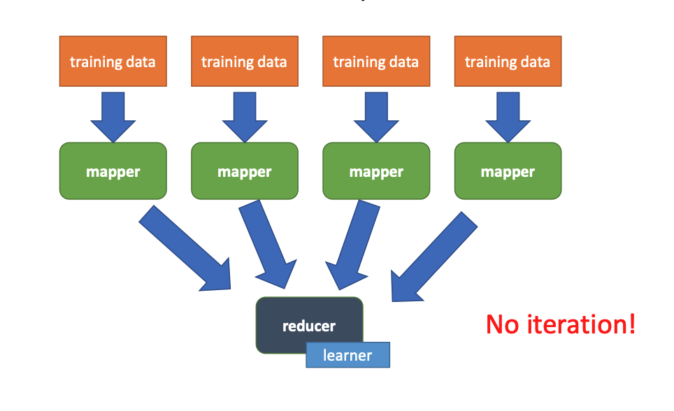
MapReduce: Multiple Models (Ensemble)

• Parallel Learning: Each mapper holds a copy of the current parameters in memory and trains its own local model based on its data partition.
  • Mapper → train → output model weights
  • Reducer:
    • may combine models
    • or just store them
• Cleanup: Each mapper outputs a completed model.
• Ensemble Learning: Multiple independent models are combined to improve performance.

Ensemble Learning Principles

Ensemble learning combines multiple independent models to create a more robust predictor.

• Combination Methods: Predictions can be merged through Voting (for classification) or by Merging Models (averaging weights for linear/sigmoidal functions).
• Why it Works: It reduces variance and relies on the hope that errors between independent models are not correlated.

Spark for Iterative Learning

Apache Spark is significantly more efficient than Hadoop for machine learning because it can cache data in memory, eliminating the need to reload it from disk for every iteration.

Spark Logistic Regression Code Snippet

The following Scala-like code illustrates a simplified training loop in Spark:

// Load and cache training points
val points = spark.textFile(...).map(...).cache()
var w = ... // initial weight vector

for (i <- 1 to ITERATIONS) {
  // Compute the gradient across all partitions
  val gradient = points.map { p =>
    val score = p.x * w
    val y = 1 / (1 + exp(-score))
    p.x * (y - p.y)
  }.reduce((a, b) => a + b)

  // Update the weight vector
  w -= gradient * LR
}

• Efficiency: Caching data and avoiding "shuffles" makes this faster than MapReduce.
• Scaling Limit: Even in Spark, shipping the gradient for a model with millions of parameters to the driver node can eventually become a bottleneck.

Stochastic Gradient Descent (SGD) at Scale

To further scale, Online Stochastic Gradient Descent can be used:

• Subset Processing: Instead of the full dataset, the gradient is computed for a random subset or even one element at a time.
• High-Quality Iterations: While individual iterations are "lower quality" than full-data methods, they allow for thousands of times more iterations for the same amount of work.

Machine Learning Model Evaluation and Validation

The Pitfall of Overfitting

A common mistake is evaluating a model only on the data it was trained on.

• Definition: Overfitting occurs when a model learns the "noise" or specific quirks of the training set rather than the underlying patterns.
• The Symptom: A model might have zero loss on training data but perform poorly on a new test dataset.
• Mitigation: Using larger, more representative training sets and techniques like "checkpointing" (saving the model at various stages of training) can help.
  • Epoch: 1 pass through the training data
  • Usually you checkpoint every \(X\) epochs, the smaller \(X\) the better, but also the more HDD space you use

Evaluation Metrics

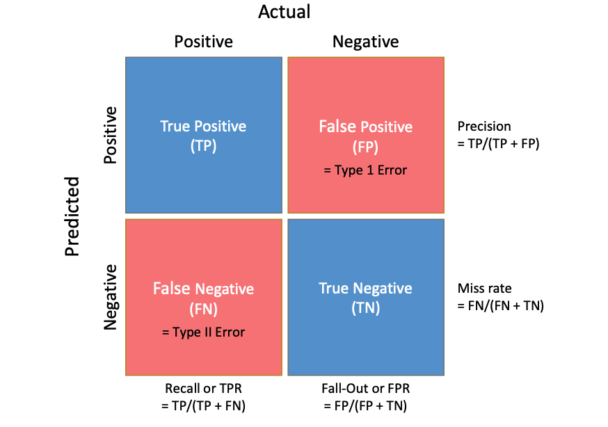
Accuracy is often not a sufficient measure of success, especially in imbalanced datasets. Instead, practitioners use a Confusion Matrix to track four key outcomes:

• True Positive (TP): Correctly predicted "Yes".
• True Negative (TN): Correctly predicted "No".
• False Positive (FP): "Type 1 Error"—predicting "Yes" when it is actually a "No".
• False Negative (FN): "Type II Error"—predicting "No" when it is actually a "Yes".

Derived Statistical Measures

From these counts, several critical metrics are calculated:

• Precision: How many of our "Yes" predictions were actually correct?

\[ Precision = \frac{TP}{TP + FP} \]

• Recall (True Positive Rate): How many of the actual "Yes" cases did we successfully find?

\[ Recall = \frac{TP}{TP + FN} \]

• Miss Rate: How many "Yes" cases did we overlook?

\[ Miss Rate = \frac{FN}{FN + TN} \]

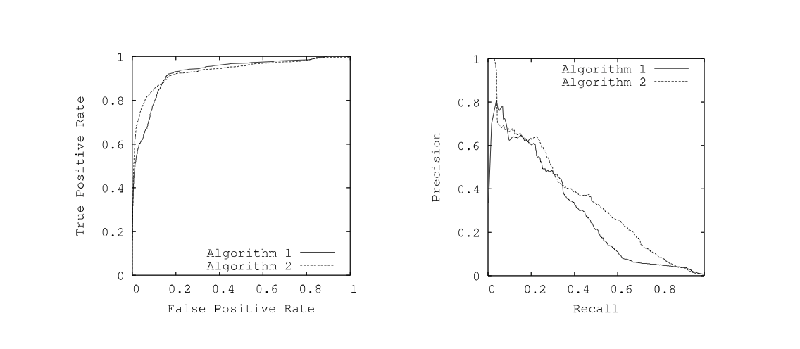
Threshold Invariant Evaluation: ROC and PR Curves

Since many classifiers output a probability rather than a hard label, their performance depends on the chosen "threshold" (e.g., is >50% enough to call it Spam?).

• ROC Curve: Graphs Recall (True Positive Rate) vs. Fall-Out (False Positive Rate).
• PR Curve: Graphs Precision vs. Recall.
• AUC / ROCA: The "Area Under the Curve" provides a single number representing the model's quality across all possible thresholds. A ROCA of 1.0 is a perfect predictor; 0.5 is equivalent to random guessing.

Cross-Validation and Testing

To trust that a model will work in real-time "live" scenarios, it must be validated "offline" using data it has never seen.

Cross-Validation Techniques

• Holdout Method: The dataset is split into a Training Set and a Testing Set (the "Holdout"). However, the less data we train on, the worse the model; the less we test on, the less we trust the results.
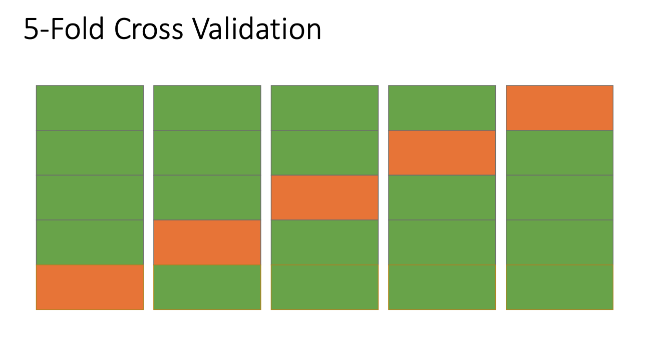
• K-Fold Cross Validation: This provides a more robust solution by rotating the data.
  1. Divide the data into K subsets (folds).
  2. Repeat the process K times.
  3. In each iteration, use one subset for testing and the other K-1 subsets for training.
  4. Benefit: Every data point is used for validation exactly once and for training \(K-1\) times.
  5. Outcome: You end up with K independent models that can be merged or used for "voting" to provide more confident predictions.

Online Testing (A/B Testing)

• A/B Testing (Online): Used to compare two alternatives (Option A vs. Option B) by splitting traffic (\(X\%\) vs. \(100-X\%\)) and gathering metrics.
  • In marketing: Checks for a single variable.
  • In medicine: Often "Double Blind" to prevent bias.
• ML Evaluation Workflow:
  • Step 1: Offline training and evaluation (holdout sets, cross-validation).
  • Step 2: Online A/B testing against current best-practice models or other methods.
  • Iteration: Returning to offline training if online results are unsatisfactory.

Locality Sensitive Hashing (LSH) and Similarity Search

Problem Definition and Objectives

• Near Neighbors Problem: Given a set of objects \(S\) and a distance function \(D(a, b)\), find all unordered pairs \((a, b)\) such that the distance is below a maximum threshold \(t\) (\(D(a,b) \le t\)).
• Core Objective: Given high-dimensional datapoints \(x_1, x_2, ... x_n\), find all pairs \((x_i, x_j)\) such that \(d(x_i, x_j) < s\).
• Efficiency Goals:
  • Naïve Approach: Computing distances for all pairs results in \(O(n^2)\) complexity, which is inefficient for big data.
  • Target Complexity: Achieving \(O(n)\) is the goal for practical machine learning and big data applications.
• Identical Item Search: Finding identical items can be done in \(O(n)\) using a hash table by only comparing collisions rather than all pairs.

Similarity Measurement Domains

• Document Similarity: Important for Information Retrieval (IR) to detect near-duplicates in mirrors of Usenet content or news sites where articles may have minor edits or different headers/footers.
• Image Similarity: Can be measured in two distinct ways:
  • Visual Similarity: Tricky to model as it requires human vision/cognition or complex neural networks.
  • Subject Similarity: Identifying "what is in the image" using inverted indices or neural networks like BLIP.
• Protein Folding: Finding similar sequences in databases is not as simple as Hamming distance because not all mutations are equal (e.g., Leucine to Isoleucine is nearly identical, while Leucine to Lysine is very different).

Dimensionality Reduction and Embeddings

• High-Dimensional Challenges: Feature vectors can be too large to work with effectively. For example, a 140-character text message has \(256^{140}\) possible states, resulting in a sparse vector.
• N-gram Embedding: Using character 4-grams reduces the space to \(256^4\), which is still large and sparse. (Note: A document can be represented as a set of its overlapping n-gram sequences. Optimal values are 4-5 bytes for short text, 8-10 for long text; or 2-3 words for short text, 3-5 for long text).
• Reducing Dimensions: To further reduce \(n\)-grams, they can be hashed modulo a large prime (e.g., \(mod\ 1,000,009\)).
• Collision Management: At a scale of \(1M\) dimensions compared to \(4B\), collisions are considered rare enough to ignore in certain assignments.

Locality Sensitive Hashing (LSH) Mechanism

• Mechanism Comparison:

For \(X, X'\) such that \(d(X, X’)=c\)

Feature	Normal Hash Function	LSH Hash Function
Output Behavior	If \(h(X)\) is known, there is no way to predict \(h(X')\)	Items that are "close" in input space have hash codes that are "close" on average
Distance Correlation	No predictable relationship between \(d(X, X')\) and \(d(h(X), h(X'))\)	\(E[d_{hash}(h(X), h(X'))] = c\), where \(c\) is the input distance
- LSH Implementation Notes:
- The similarity in hash codes is an expected value; individual results may vary.
- The distance metric used for hash codes (\(d_{hash}\)) is different from the original metric (\(d\)) because the hash function may return different data types.
- Ideally, the distribution of these distances should be a normal distribution.

Principles

• Core Logic: An LSH hash function \(h(x)\) ensures that items "close" in the input space result in hash codes that are "close" on average.
• Implementation (Scalar):
  1. Construct a hash table.
  2. Define buckets of width \(w\) that overlap so single items can reside in multiple buckets.
  3. Determine that most values within distance \(c\) will share at least one bucket, while values exceeding distance \(c\) will not.

Jaccard Similarity and Distance

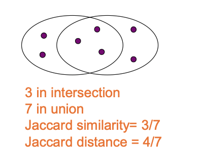
• Similarity: Defined as the size of the intersection divided by the size of the union of two sets: \(sim(C_1, C_2) = \frac{|C_1 \cap C_2|}{|C_1 \cup C_2|}\).
• Distance: Calculated as the complement of similarity: \(d(C_1, C_2) = 1 - sim(C_1, C_2)\).

• Multisets: For embeddings where element counts matter, Jaccard definitions are adjusted: Union (\(C=A\cup B\)) uses \(\max(A[k], B[k])\) and Intersection (\(C=A\cap B\)) uses \(\min(A[k], B[k])\), where \(|A|\) is the sum of the counts for all keys in \(A\).

Min-Hashing for Jaccard Distance

• Target Application: Min-Hashing is the specialized LSH technique for Jaccard distance.
• Algorithm Mechanism:
  • Let \(C\) be a set of n-grams (numbered as integers).
  • Apply a random permutation (or random enumeration function) \(\pi\) to the universe of elements.
  • The hash value \(h(C; \pi)\) is the minimum value in the set under that permutation: \(h(C; \pi) = \min_{i \in C} \pi(i)\).
• Statistical Property: Highly similar sets will have \(h(C_1) = h(C_2)\) with high probability, whereas highly dissimilar sets will not.

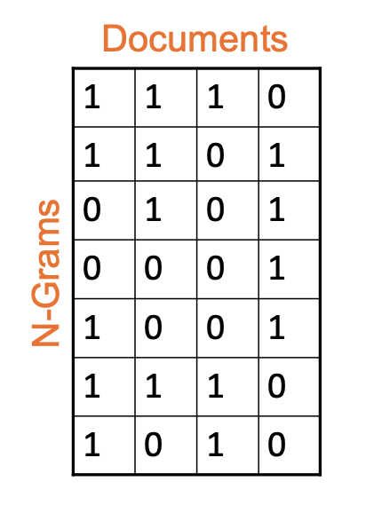
Matrix Representation and Signatures

• Structure: A collection of documents is represented as an Input Matrix where rows correspond to unique n-grams in the universe and columns represent individual documents.
• Binary Values: An entry \((i, j)\) is 1 if n-gram \(i\) is present in document \(j\), and 0 otherwise.
• Goal: The objective is to compute a signature for each column such that the size of the signature is significantly smaller than the original column (\(|sig| \ll |col|\)), while preserving similarity.

Permutations and Signature Generation

• Permutation Definition (\(\pi\)): A rule where each n-gram is moved to a new index in a random reordering.

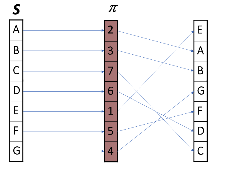
• Min-Hash Property: The probability that two sets have the same min-hash value (\(h(C_1; \pi) = h(C_2; \pi)\)) is exactly equal to their Jaccard similarity.
• Signature Generation:
  • Generate \(K\) independent permutations. For each document \(C\), the \(i\)-th entry of the signature is the min-hash defined by the \(i\)-th permutation: \(Sig(C)[i] = h(C; \pi_i)\).
  • This results in a smaller data footprint (e.g. \(K=100\) gives 400 bytes).
  • Using multiple hash functions allows the distribution to converge on a normal distribution via the Central Limit Theorem.

Similarity and Example Calculation

• Signature Similarity: Measured as the percentage of entries that are equal.
• Expectation: \(E[sim(Sig_1, Sig_2)] = sim(C_1, C_2)\).
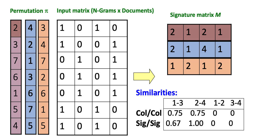
• Example Process:
  1. Use an Input Matrix (N-Grams x Documents) and multiple permutations \(\pi\).
  2. For each permutation, identify the first row (the smallest index in the permutation) that contains a 1 for that document.
  3. Record that row's permutation value in the Signature Matrix \(M\).
  4. Compare the resulting column similarities (Col/Col) against the signature similarities (Sig/Sig) to estimate document likeness.

Candidate Pair Identification

• Definition: Documents A and B are categorized as a "candidate pair" if their MinHash similarity is greater than or equal to a target threshold \(s\).
• Efficiency Challenge: A purely signature-based comparison theoretically still requires all pairwise comparisons between documents.
• LSH Requirement: To achieve efficient scaling, LSH requires the use of a hash table rather than just comparing codes.

MinHash Table Implementation and Logic

• Vector Challenge: A MinHash signature is an \(n\)-vector, which is more complex to assign to buckets than a scalar hash code.
• Implementation Strategies:
  1. N-dimensional table: Using a secondary hash function on the signature vector to map it to a 1-dimensional table.
  2. Independent tables: Using \(n\) independent 1-dimensional tables.

• Implementation Code Snippet:

  sig[C][i] = ∞ for all C, I
  for each row index j in each column C:
      if C[j]:
          for each hash function index i:
              sig[C][i] = min(sig[C][i], h_i(j))
  

• The Prohibitive Nature of Permutations: Calculating \(n!\) permutations is computationally impossible. Instead, k-universal hash functions are used as a "close enough" alternative to pick the "smallest" element uniformly.

The Banding Technique

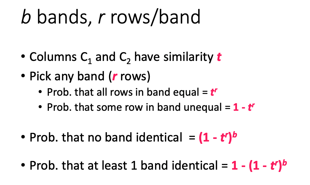
• Mechanism: The signature vector is sliced into \(b\) equal-sized "bands" consisting of \(r\) values each.
• Bucket Assignment: There are \(b\) separate 1-dimensional tables.
• Candidate Criteria: A pair \((A, B)\) is a candidate if they collide in any of the \(b\) tables.
• Trade-off Resolution:
  • High-similarity documents (e.g., 80%) might not have identical full signatures but likely share at least one band.
  • Low-similarity documents (e.g., 10%) are unlikely to share an entire band, reducing false positives.

Banding Parameters and Matrix Partitioning

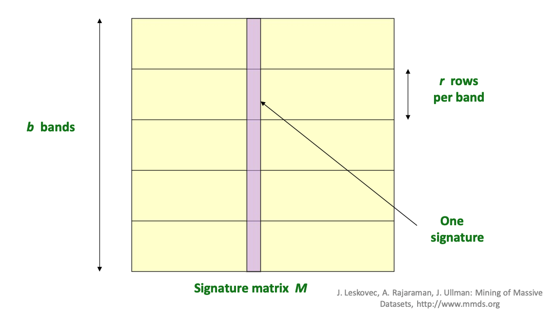
• Matrix Partitioning: The Signature Matrix \(M\) is horizontally partitioned into \(b\) bands.
• Band Structure: Each individual band contains \(r\) rows per band.
• One Signature: A single vertical column represents one document's signature across all bands.

Hashing Bands and Candidate Pairs

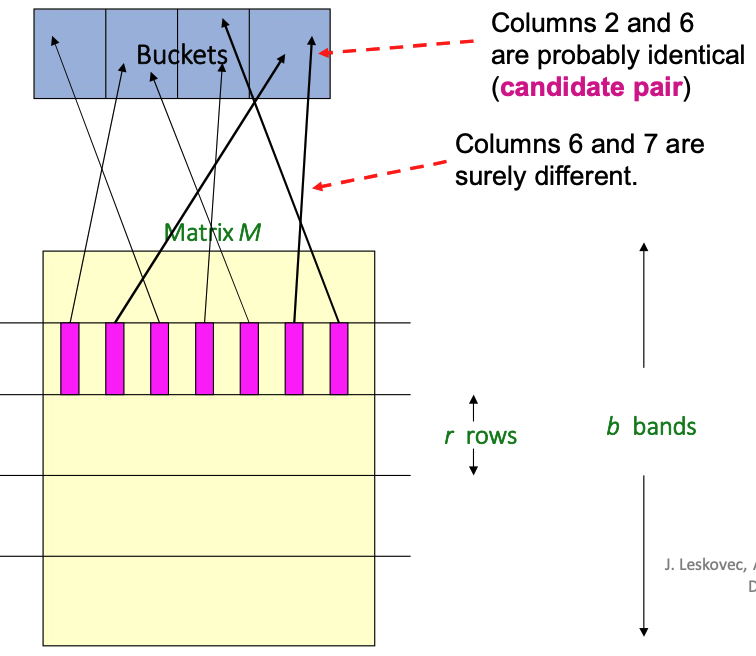
• Bucket Mapping: Columns (documents) in the signature matrix \(M\) are hashed into buckets based on their values within a specific band.

• Candidate Pair Identification:

  • Similar Columns: If columns (e.g., 2 and 6) have identical values within at least one band, they hash to the same bucket and are considered a candidate pair.
  • Dissimilar Columns: If columns (e.g., 6 and 7) differ across all bands, they are highly unlikely to collide and are dismissed.

  

Banding Parameters and Goals

• Example Scenario: For a collection of 100,000 documents, signatures are composed of 100 integers (rows), totaling 40 MB of data.
• Configuration: Choosing \(b = 20\) bands and \(r = 5\) rows per band creates a specific probability curve for identifying pairs.
• Objective: The goal is to identify all pairs of documents with at least \(s = 0.8\) similarity.

Probability Analysis for Similar and Dissimilar Pairs

• High Similarity Case (\(s = 0.8\)):
  • Probability of being identical in one specific band: \((0.8)^5 = 0.328\).
  • Probability of not being identical in any of the 20 bands: \((1 - 0.328)^{20} = 0.00035\).
  • Result: Only about 1/3000th of truly similar pairs are missed (false negatives), finding 99.965% of target documents.
• Low Similarity Case (\(s = 0.3\)):
  • Probability of being identical in one specific band: \((0.3)^5 = 0.00243\).
  • Probability of being identical in at least one of 20 bands: \(1 - (1 - 0.00243)^{20} = 0.0474\).
  • Result: Approximately 4.74% of dissimilar docs mistakenly become candidate pairs (false positives).

LSH Trade-offs and Tuning

• Tuning Parameters: To balance performance, one must strategically pick:
  1. The number of Min-Hashes (total rows in \(M\)).
  2. The number of bands \(b\).
  3. The number of rows \(r\) per band.
• Effect of Parameter Shifts:
  • Decreasing the number of bands (e.g., to 15) causes false positives to go down but false negatives to go up.